Numerical measures: three questions
Where do values lie?
Location Mean, median, mode, percentiles, quartiles
How far apart are values?
Variability / dispersion Variance, standard deviation, range, IQR
What about asymmetry and extremes?
Shape Skewness, kurtosis
Describe a typical balance, its spread, and the shape of the distribution.
This restores the original Numerical measures overview. Mean, median and mode describe central tendency; percentiles and quartiles describe positions throughout the ordered data. Variability measures dispersion, while skewness and kurtosis describe asymmetry and the contribution of extreme observations. The same mean can occur with very different spreads or shapes.
Allow 40 minutes for this section, including the seven-minute balance exercise, a two-minute Wooclap comparison of branch review times and about five minutes for the three shape slides. Develop location first, then use that vote to motivate variability. Work through one sample variance calculation and explain the denominator graph without deriving its expectation in class. Read the skewness and kurtosis formulas through their meaning: the third power retains direction; the fourth power emphasises extremes on either side.
Location: Mean
The arithmetic mean is the sum of the values divided by their number.
\(\displaystyle\bar{x}=\frac{1}{n}\sum_{i=1}^{n}x_i\) \(\displaystyle\mu=\frac{1}{N}\sum_{i=1}^{N}x_i\)
For the six campaign balances: \(\bar{x}=€3{,}912/6=€652\) .
Uses every value, so large balances pull the mean upwards.
Balances deviations: \(\sum_{i=1}^{n}(x_i-\bar{x})=0\) .
Connects to the total: total balance \(=n\bar{x}\) .
The six values are 2143, 29, 2, 1506, 1 and 231 euros. Their sum is 3912, so their mean is 652. Read x-bar and mu aloud and connect them to the preceding statistic/parameter slide. N is the size of the defined population; n is the number of observations in the sample. Both formulas use the same arithmetic operation on different sets of values.
The six rows are an excerpt of the UCI file. Calculating their mean describes those balances; generalising requires a sampling argument. The mean is useful for totals and aggregate exposure. Its sensitivity to extreme values will be explored in the balance exercise.
Location: Mode
The mode is the value or category with the greatest frequency.
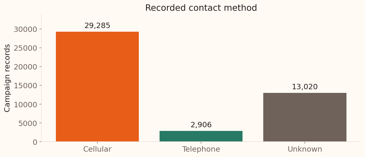
For the 45,211 campaign records:
Cellular
29,285
Unknown
13,020
Telephone
2,906
Mode = Cellular . A mode can summarise categorical as well as numerical data.
Tied highest frequencies can give more than one modal value. If all numerical observations occur once, a mode usually provides little useful summary. Unknown is a recorded missing-information category and remains visible in the frequency table. A mean contact method has no numerical meaning, which makes this a useful example of choosing a summary from the variable type.
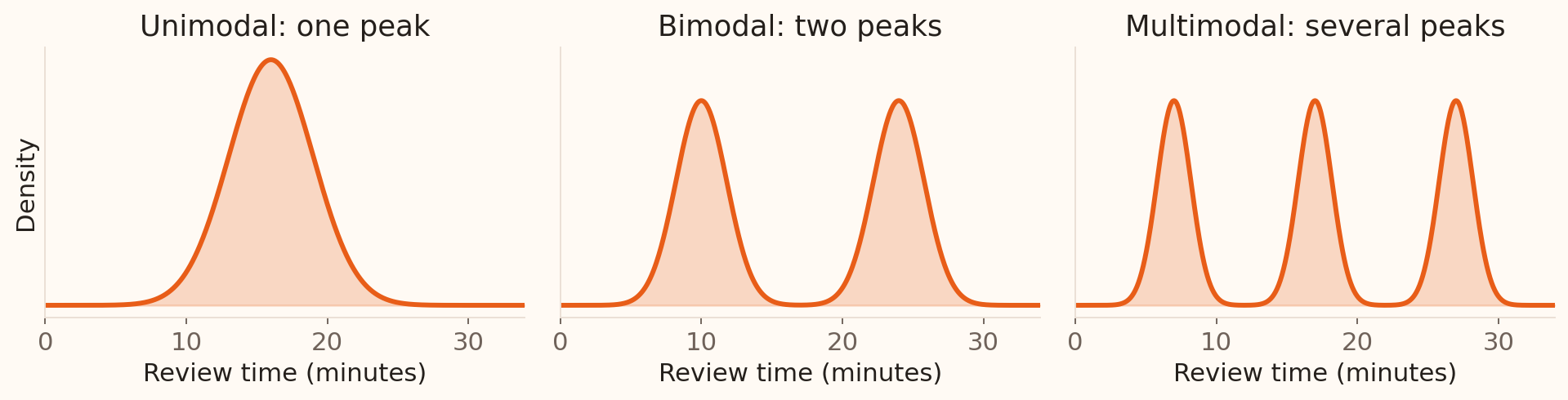
One mode or several?
For a numerical distribution, modes are local peaks .
Several peaks can suggest different customer groups or review processes.
Illustrative densities generated in Python; these are hypothetical review times.
This restores the original unimodal/bimodal/multimodal illustration. Bimodal distributions have two local peaks; the peaks need not have equal height. For example, combining routine and complex applications can create distinct peaks in review times. Inspect the underlying groups before explaining a peak. Histogram bins and density smoothing can change which peaks are visible, as discussed in Statistical Graphics.
What changes when one balance changes?
Use the six recorded balances: €2,143, €29, €2, €1,506, €1, €231 .
Calculate the mean and median.
In a hypothetical version, replace €2,143 with €21,430.
Predict which summary changes most, then check your calculation.
Which result would you use for a typical customer, and which for the total balance?
Allow 7 minutes within the centre-and-spread block: 3 minutes calculating in pairs, 2 minutes comparing, 2 minutes debrief. Original sum €3,912, mean €652, median (29+231)/2=€130. New sum €23,199, mean €3,866.50; median remains €130. The mean responds because it uses magnitudes; the median depends on the central ordered observations. The original six values are from the UCI data; the replacement is explicitly hypothetical. The total equals n times the mean. This exercise develops the earlier formulas rather than introducing a new summary.
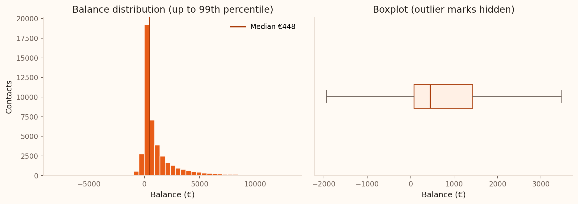
Mean or median? Real balances
Mean = €1,362 ; median = €448 .
For a typical recorded customer , lead with the median and the distribution.
For the total recorded balance , use the mean multiplied by the record count.
Source: UCI Bank Marketing . Figure generated from all 45,211 records; histogram truncated at the 99th percentile and boxplot outlier marks hidden for legibility.
The plot shows the long upper tail that pulls the mean above the median. The mean is 1362.272… before rounding, so use the unrounded value for an exact total. The median is useful for describing a typical balance, while the mean retains the contribution of large balances to the aggregate. The choice follows the banking question.
Location: Percentiles
The \(p\) th percentile\(p\%\) of the observations at or below it.
Illustrative banking example: the 90th percentile of application review time is 45 minutes .
About 90% of recorded reviews took 45 minutes or less; about 10% took longer.
The percentile level tells us where a value sits in the ordered data.
The percentile value has the variable’s units: here, minutes .
This restores the standalone percentile explanation, replacing the original GMAT example with banking operations. A high percentile can describe slow service or large losses that a typical value misses. The 90th percentile is a position in the distribution, not 90% of the maximum observed time. Ties and finite-sample interpolation conventions affect the exact share at or below a reported percentile, so the wording uses approximately. The 45-minute value is illustrative.
Location: Quartiles
Quartiles are the 25th, 50th and 75th percentiles ; \(Q_2\) is the median.
The middle 50% lies between \(Q_1\) and \(Q_3\) .
The diagram uses ordered position, so equal-width bands represent approximately equal shares of records. It does not imply that the monetary gaps between quartiles are equal. The recorded quartiles use pandas’ default linear interpolation. Other software conventions can give slightly different sample quantiles, especially for small datasets. Introduce the interval between Q1 and Q3 here; its numerical width is the interquartile range.
Same mean, same spread?
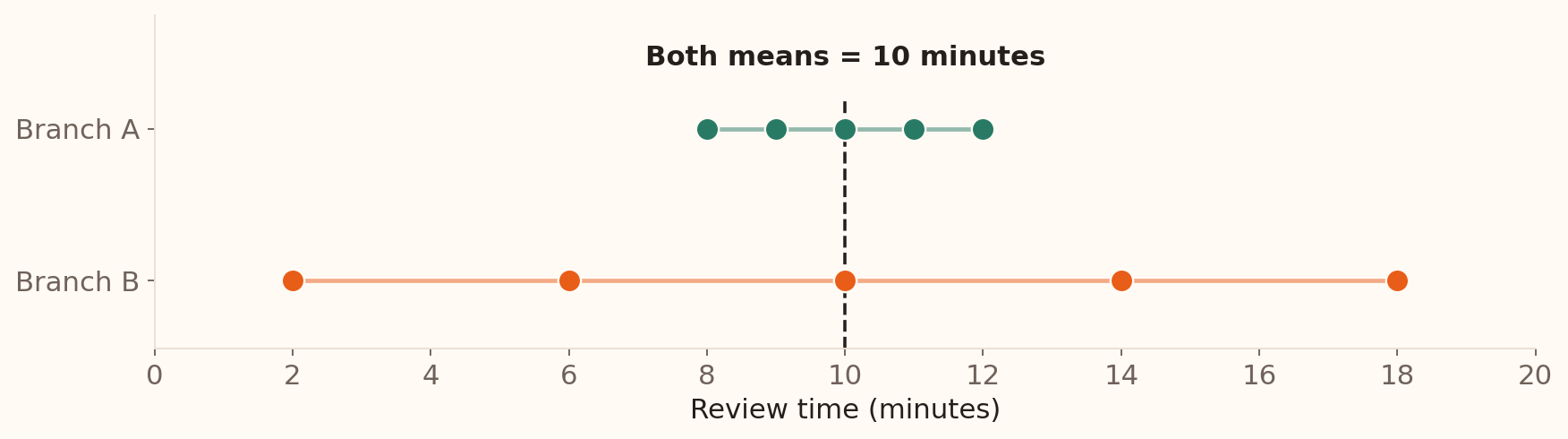
These illustrative branches both have a mean review time of 10 minutes. Which has more consistent observed review times?
A
8, 9, 10, 11, 12
B
2, 6, 10, 14, 18
Branch A
Branch B
Both are equally consistent because their means are equal.
We cannot compare consistency from these observations.
Format: multiple choice, one answer. Correct: option 1. Allow 2 minutes within Centre & Spread: 45 seconds to compare and vote, then 75 seconds to explain using the next slide. Branch A’s observations lie closer to their shared mean of 10 minutes. Its range is 4 minutes, compared with 16 minutes for Branch B. This is the existing branch-comparison discussion delivered as a poll. Students can answer by inspecting the values before learning the variability formulas.
Measures of variability
Variability , or dispersion, describes how far the observations spread out.
Variance and standard deviation: use deviations from the mean.Range and IQR: measure the width of all or part of the data.
The two branches are hypothetical samples of five application reviews each. Use this plot to debrief the preceding vote before introducing the formulas. Both means and medians are 10 minutes. Branch A has range 4 minutes and sample SD about 1.58 minutes; Branch B has range 16 minutes and sample SD about 6.32 minutes. Equal means therefore leave an important operational difference unexplained. Reuse Branch B for the worked variance calculation.
Variability: Variance and SD
Variance uses squared deviations from the mean. Standard deviation (SD) is its square root.
Variance
\(\displaystyle\sigma^2=\frac{\sum_{i=1}^{N}(x_i-\mu)^2}{N}\) \(\displaystyle s^2=\frac{\sum_{i=1}^{n}(x_i-\bar{x})^2}{n-1}\)
SD
\(\sigma=\sqrt{\sigma^2}\) \(s=\sqrt{s^2}\)
For review times, variance is in minutes squared ; SD is in minutes .
SD expresses spread around the mean in the original measurement units.
The population formula averages squared deviations over every value in a defined finite population. The sample formula uses the observed mean and the n−1 correction; the next two slides develop its calculation and rationale. Squaring makes all contributions non-negative and gives larger deviations greater weight. Variance and SD are zero when all observations are equal, and both are sensitive to extreme values. Sample variance requires n greater than one.
The sample SD describes the spread of observations. Its units are euros for balances and minutes for review times. The standard error of an estimated mean is a different quantity, introduced with sampling distributions later.
Calculating variance and SD
For Branch B’s five review times, \(\bar{x}=(2+6+10+14+18)/5=10\) minutes.
2
−8
64
6
−4
16
10
0
0
14
4
16
18
8
64
Total 0 160
\[s^2=\frac{160}{5-1}=40\text{ minutes}^2,
\qquad s=\sqrt{40}\approx6.32\text{ minutes}.\]
Work from the raw values to deviations, squared deviations, variance and SD. Ask why simply averaging the signed deviations would fail: they sum to zero. The same calculations for Branch A give sum of squared deviations 10, sample variance 2.5 and sample SD about 1.58 minutes. Branch B’s SD is four times Branch A’s, while its variance is sixteen times as large.
Here the five reviews are a sample. If the question instead concerned exactly these five reviews as the entire population, their population variance would be 160/5 = 32 minutes squared and their SD about 5.66 minutes. The full worked calculation is reproduced by scripts/build_teaching_figures.py –location-spread-only.
Why divide by \(n-1\) ?
Deviations from \(\bar{x}\) sum to zero: only \(n-1\) vary freely
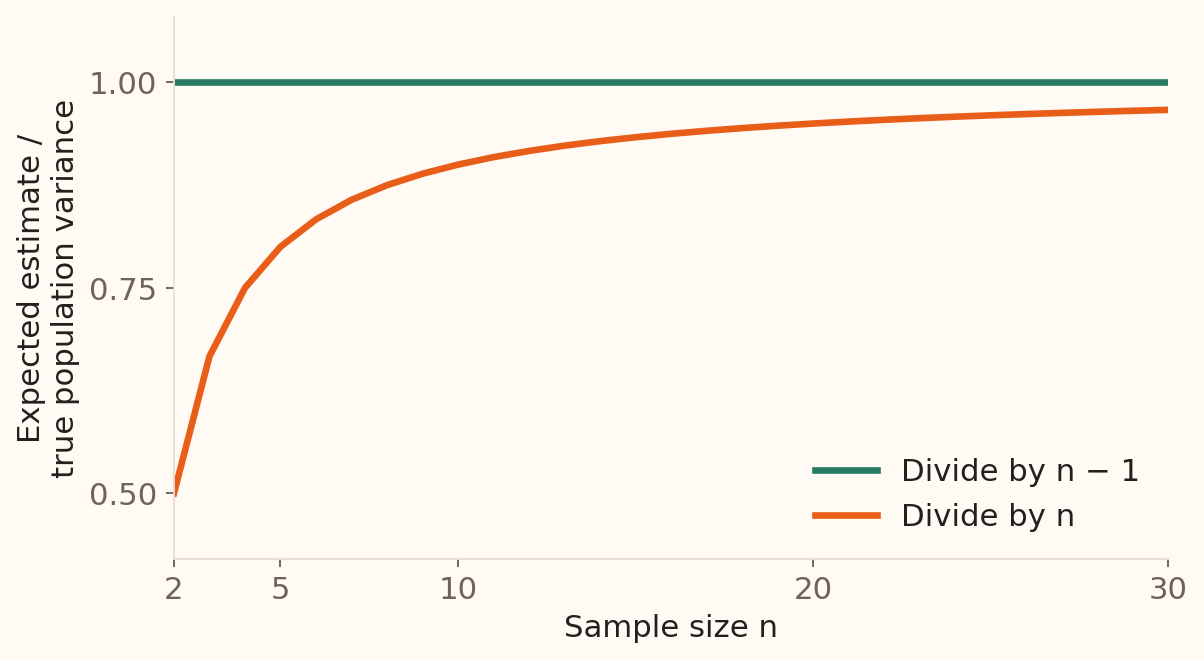
Dividing by \(n\) underestimates population variance on average .
Dividing by \(n-1\) corrects this bias.
An unbiased estimate is correct on average over repeated samples: \(\mathbb{E}[s^2]=\sigma^2\) .
Theoretical expectations for independent observations from a common distribution with positive finite variance.
This replaces the original sample_variance_converge graphic with exact expectation curves. Under independent, identically distributed sampling with finite variance, E[sum (Xi−Xbar)^2] = (n−1)σ². Dividing by n therefore has expectation (n−1)σ²/n, while dividing by n−1 gives expectation σ². The graph plots these expectations relative to σ². It does not show the variance from one realised sample. Individual estimates fluctuate, and the n−1 correction does not make each estimate exact. The sample SD itself is not generally unbiased.
The earlier 800-customer example uses sampling without replacement from a finite population. In that setting, s² is unbiased for the finite-population variance defined with denominator N−1. If σ² is defined with denominator N as on the preceding population-formula slide, E[s²] = Nσ²/(N−1). The expectation graph here explicitly uses the independent-sampling model; leave this finite-population distinction for follow-up if needed.
Variability: Range and IQR
Range \(102{,}127-(-8{,}019)=110{,}146\) Full span; determined by two extremes
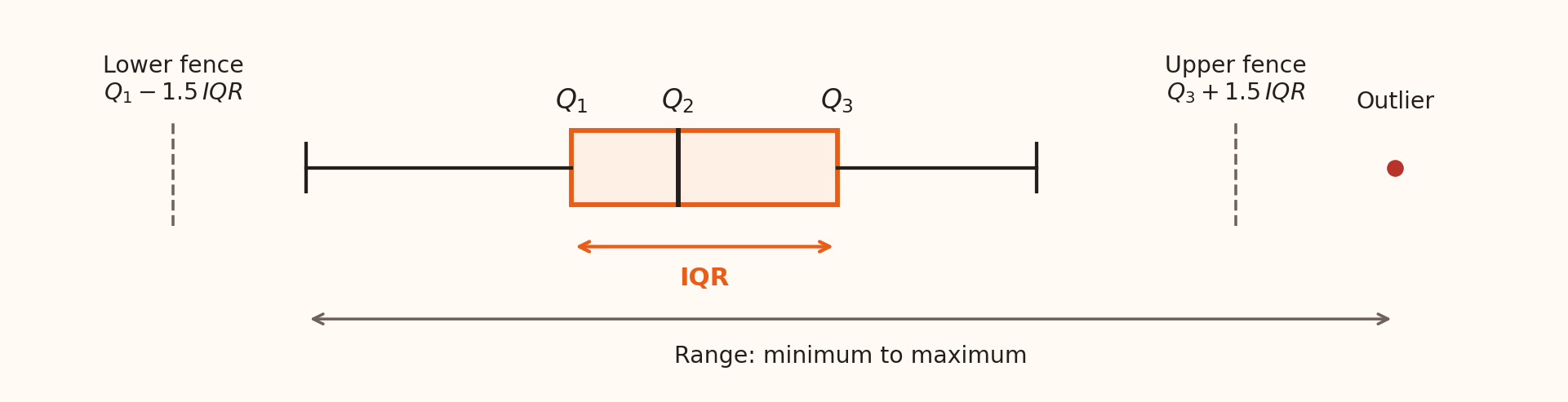
IQR \(Q_3-Q_1=1{,}428-72=1{,}356\) Width of the middle 50%
The IQR is resistant to extreme values; the range is highly sensitive to them.
The diagram illustrates the boxplot convention, not the numerical scale of the bank data. Its IQR is the box width. Whiskers reach observed values inside the fences, while the range extends from the smallest to the largest observation, including any plotted outliers. The full-data balance range is 102127−(−8019)=110146 euros; IQR is 1428−72=1356 euros. The contrast shows how much the extremes add beyond the central half of the balances.
Outliers: a flag, not a verdict
An outlier is unusually small or large for the variable and setting.
IQR rule Below \(Q_1-1.5\,IQR\) or above \(Q_3+1.5\,IQR\)
Based on the central half of the data
Three-SD rule Outside \(\bar{x}\pm3s\)
A heuristic for roughly bell-shaped data
For recorded balances, the IQR fences are −€1,962 and €3,462 .
Investigate recording errors, unusual genuine cases and different subgroups.
The IQR rule uses 72−1.5×1356=−1962 and 1428+1.5×1356=3462 euros. These are calculated cut-offs, not necessarily observed values. In a boxplot, each whisker stops at the most extreme observation within its fence. A point exactly on a fence is inside it.
The original slides also offered a three-standard-deviation screen. Its interpretation depends on distributional shape; skewed or heavy-tailed data can produce many legitimate observations beyond that interval. For an exactly normal population, about 0.27% lies outside μ±3σ; using an estimated mean and SD does not produce an exact test with that rate. Check the measurement and banking context before deciding how to handle a flagged value.
A five-number summary
Minimum
−8,019
\(Q_1\) 72
Median
448
\(Q_3\) 1,428
Maximum
102,127
For the central balances, report median €448 and IQR €1,356 ; report the extremes alongside them.
Connect measures of location and variability: the median locates the centre, IQR describes the central spread, and the minimum and maximum preserve information about the full extent. Negative balances may reflect overdrafts or other legitimate account states; check the variable definition and source records. Retain a distribution plot because these five numbers do not reveal every group or peak.
Shape matters for risk
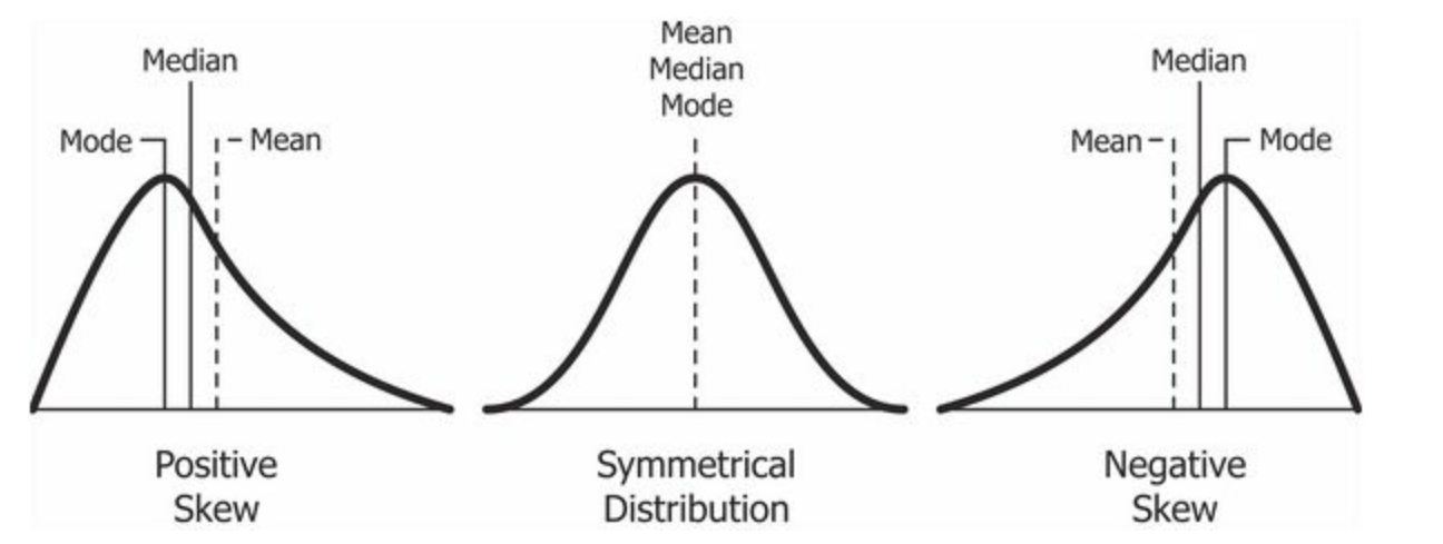
Name the long tail : right = positive skew; left = negative skew.
For risk management, inspect the adverse tail: right for losses; left for returns .
Schematic reused from the original Week 2 slides; the marked order describes these examples.
Begin the five-minute shape discussion with the original three-panel figure from SOA-week2.tex, then use the next two slides for the formulas and the contrast with kurtosis. Read the marked positions from left to right: mode < median < mean for the positive-skew example; mean = median = mode for the symmetric example; mean < median < mode for the negative-skew example. In these examples, the mean lies towards the long tail. Name skewness by the long tail, rather than the side containing the peak. Ask students to point to the long tail before naming its sign, then connect the mean-minus-median difference to Pearson’s coefficient on the next slide.
Positive skew in a loss variable directs attention to a long upper loss tail; negative skew in a return variable directs attention to large negative returns. This motivates checking adverse scenarios alongside a typical outcome and its SD.
The tail descriptions apply to the shapes illustrated. Skewness alone does not determine the probability of a gain, a loss or an extreme outcome, and mean/median/mode order is not a universal rule for all distributions. Inspect the variable, distribution and tail together when describing banking risk.
Skewness: two useful formulas
Population moment skewness: the third standardised moment.
\[\gamma_1=\mathbb{E}\!\left[\left(\frac{X-\mu}{\sigma}\right)^3\right]
=\frac{\mathbb{E}[(X-\mu)^3]}{\sigma^3}.\]
Pearson’s median coefficient: a summary calculated from the data.
\[S_{\mathrm{P}}=\frac{3(\bar{x}-\tilde{x})}{s},
\qquad \tilde{x}=\text{median},\quad s=\text{SD}.\]
Bank balances: \(S_{\mathrm{P}}\approx3(1362.27-448)/3044.77\approx0.90\) .
Both have no units; they are different summaries and their values need not agree.
Allow about two minutes. This restores both formulas from the original skewness slides. The cube inside the expectation corrects a typographical omission in SOA-week2.tex. Read expectation as a population average: cubing retains the sign of deviations, and dividing by SD cubed removes the units. The definition assumes positive finite variance and a finite third absolute moment. Symmetry implies zero moment skewness when it exists; zero skewness alone does not establish symmetry.
Use S_P for Pearson’s median coefficient so that it is clearly distinct from the moment coefficient and from excess kurtosis. In the balance calculation, the recorded mean is €1,362.2720577, median €448 and sample-convention SD €3,044.7658292. The coefficient is 0.9008299…, reported as 0.90. The euro units cancel. This coefficient is a separate descriptive measure, not an identity for the third standardised moment.
For software follow-up, define m_r = (1/n) sum (x_i−xbar)^r. The empirical moment coefficient is g_1 = m_3/m_2^(3/2); here m_2 uses divisor n. Some software reports the adjusted coefficient G_1 = sqrt(n(n−1))/(n−2) times g_1. Compare like definitions when checking results.
Kurtosis: a glance at tail risk
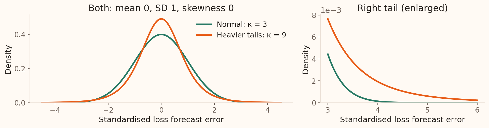
The fourth power gives large standardised deviations much greater weight.
\[\kappa=\mathbb{E}\!\left[\left(\frac{X-\mu}{\sigma}\right)^4\right],
\qquad \text{excess kurtosis}=\kappa-3.\]
Normal benchmark: \(\kappa=3\) , so excess kurtosis is \(0\) .
Same mean and SD can hide different extreme-loss risks .
Allow about two minutes. Skewness identifies asymmetry; kurtosis summarises the contribution of extreme standardised deviations on both sides. The fourth power makes a deviation of three SD contribute 81, compared with 1 for a deviation of one SD. Both measures have no units. The population kurtosis definition requires positive finite variance and a finite fourth moment. Some heavy-tailed distributions have no finite fourth moment.
The green curve is standard normal. The orange curve is a Student t distribution with five degrees of freedom, multiplied by sqrt(3/5). Both therefore have mean 0, SD 1 and skewness 0. Their kurtoses are 3 and 9; their excess kurtoses are 0 and 6. Introduce this comparison through the curves and their moments; the t family is studied later. The right panel enlarges the same densities beyond three SD. These are models of standardised forecast errors, not fitted UCI losses or measured portfolio returns.
For these particular models, the probability of exceeding the mean by three SD is about 0.135% for the normal model and 0.586% for the scaled t model. A bank using only a mean and SD can therefore miss a material difference in exposure to extreme losses. Use tail plots and adverse scenarios when assessing potential losses and financial buffers. Higher kurtosis alone does not order exceedance probabilities at every threshold or identify which tail is dangerous. Interpret the fourth moment through extremes rather than peak height alone.
For data, the unadjusted empirical kurtosis is m_4/m_2^2, with m_r = (1/n) sum (x_i−xbar)^r. Subtract 3 for excess kurtosis; software may apply a sample-size adjustment. Keep the convention explicit when comparing outputs.
Allow one minute for the existing live question and a brief explanation from a student. Use the responses to establish what students already know, then introduce each chart through its banking question. The two chart-choice guides at the end bring the examples together. The live question is maintained in Wooclap.
Bar charts: compare categories
Begin the value axis at zero.
Sort intentionally when order is not inherent.
Prefer position and length over area or 3D effects.
Source: UCI Bank Marketing . Bars show counts; a chart of group means must label that different quantity.
Line charts: change over time
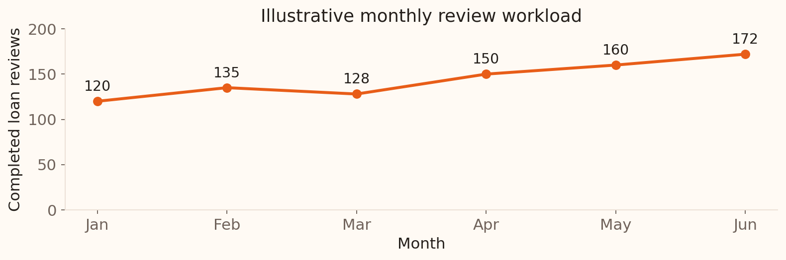
Question: How does a branch’s review workload change from month to month?
Put time on the horizontal axis; look for trends, spikes and gaps.
Illustrative monthly counts for one hypothetical branch, generated in Python.
Allow two minutes, including a brief student interpretation of the trend and the connecting lines. Each point is the number of completed loan reviews in one month: 120, 135, 128, 150, 160 and 172 from January to June. The workload generally rises, with a dip in March. The connecting line helps the eye follow time order; it does not supply observations between months. Check whether missing months, reporting changes or different month lengths affect the comparison. Six illustrative points do not establish a recurring seasonal pattern. A line chart suits an ordered time axis; separate contact categories belong in a bar chart.
Frequency distributions: group the values
A frequency distribution records the count in each group or interval.
10 to under 30
5,273
11.66%
30 to under 50
29,744
65.79%
50 to under 70
9,640
21.32%
70 to under 90
545
1.21%
90 to under 110
9
0.02%
Relative frequency = count / 45,211.
Next: turn these same age bands and counts into a histogram.
Allow two minutes for the table, followed by two minutes for its histogram. This table introduces frequency distributions as the counting step behind a histogram. Age is numerical: group the observations into intervals, count the records in each interval, then divide by the total to obtain relative frequencies. For example, 29,744 / 45,211 is about 65.79%. The intervals must cover the data without overlap; include the lower boundary and exclude the upper boundary. The next slide plots these exact age bands and counts, so students can connect each table row to one bar.
These age bands have equal width, 20 years. With equal widths, histogram heights can show counts or relative frequencies. Unequal-width bins require heights adjusted for width so that bar areas remain proportional to frequency. The later balance example demonstrates how the choice of bin width changes the visible detail.
Histograms: from the table to the plot
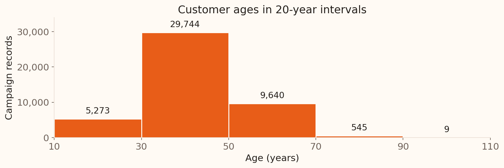
The same age bands and counts , drawn as adjoining bars.
Each bar spans a numerical interval; with equal widths, height shows count .
Source: UCI Bank Marketing , all 45,211 records; the same age bands as the preceding table.
Allow two minutes. Point from the 30-to-under-50 table row to the tallest bar: both show 29,744 records. The horizontal axis is a numerical age scale, and neighbouring intervals share boundaries. In the contact-method bar chart, bars represented separate categories; here they span numerical intervals. The broad bins show the overall age pattern, while the next slide asks how much detail a chosen bin width reveals for bank balances.
Histograms: choose the bin width
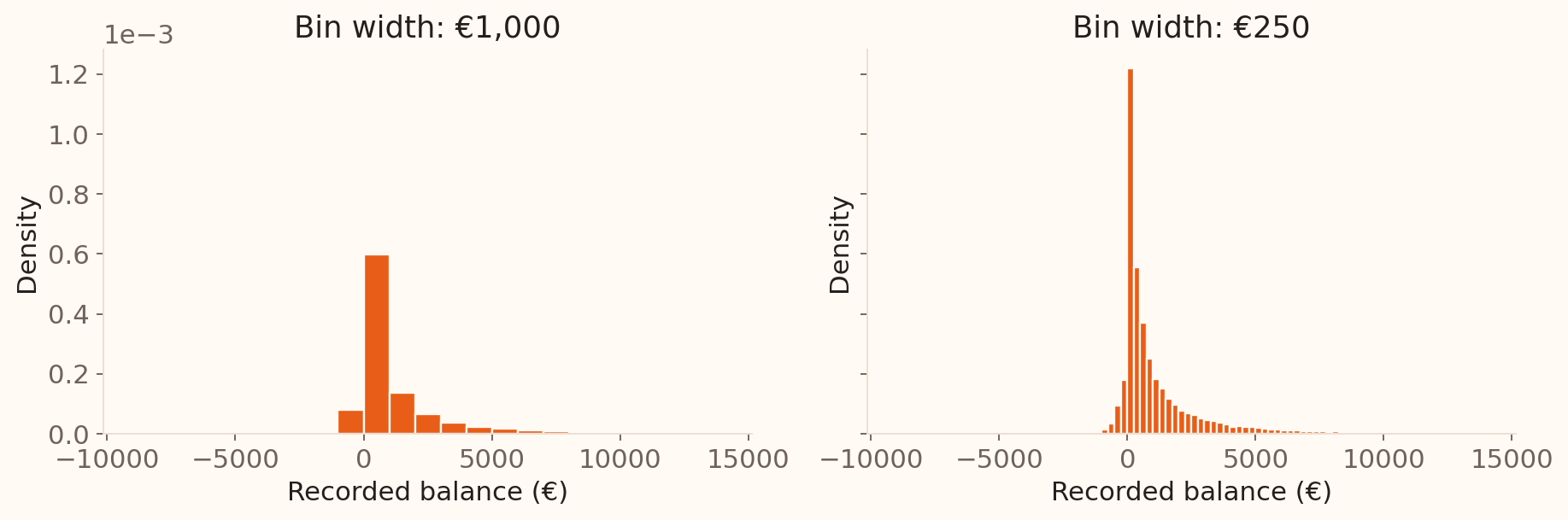
Bins that are too wide hide structure; bins that are too narrow amplify noise.
UCI Bank Marketing , balances up to the 99th percentile. Densities are normalised over that displayed subset.
Allow two minutes. Now switch from age to balance, keeping the histogram idea. Both panels contain the same displayed balances; only the bin width changes, from €1,000 to €250. A first width can be the observed range divided by a proposed number of bins, then adjusted to readable boundaries. These plots use density on the vertical axis so that bar areas represent proportions of the displayed records; density height is relative frequency divided by bin width. Narrower bins reveal more local detail but also more sampling noise.
Density plots: a smooth view
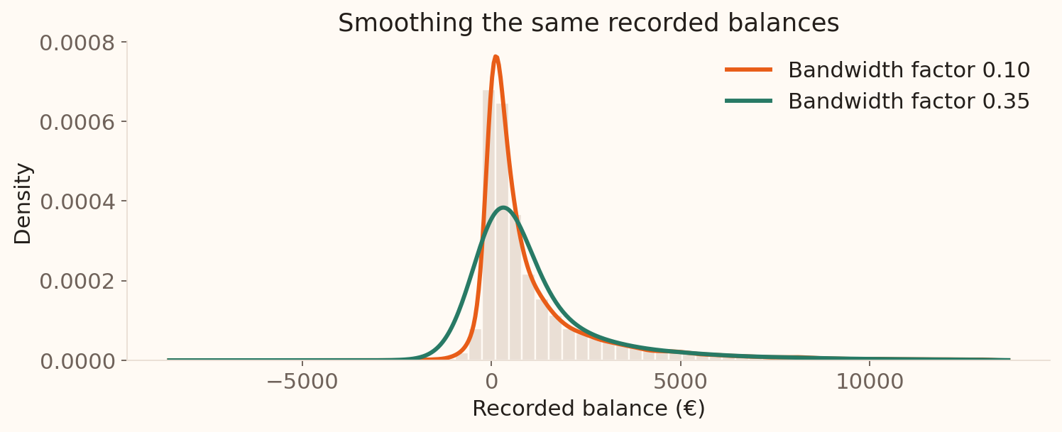
The total area is 1. Density is not a count; bandwidth controls smoothness.
UCI Bank Marketing , balances up to the 99th percentile; each fitted density integrates to one over its full support.
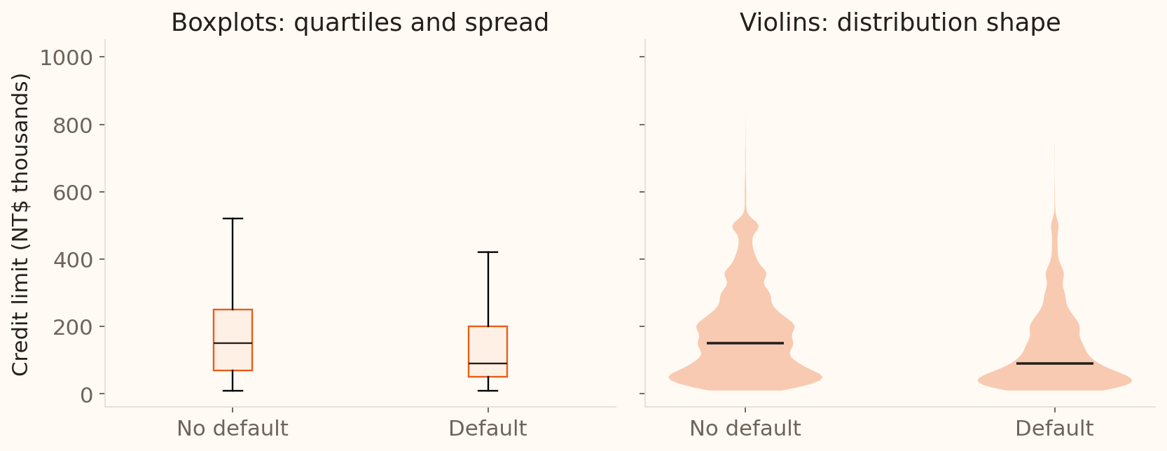
Boxplots and violins: compare groups
Boxplots summarise quartiles and spread; violins reveal the smoothed distribution shape.
Whiskers reach the most extreme observed values within the 1.5 IQR fences; they are not necessarily located exactly at the fences. A violin depends on the density bandwidth. Report group sizes alongside either chart.
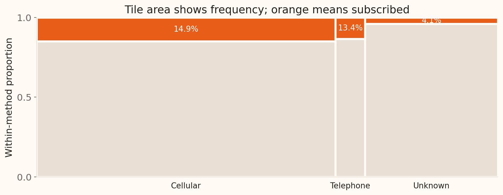
Mosaic plots: two categories
Width shows group size; orange height shows the subscription rate within each group.
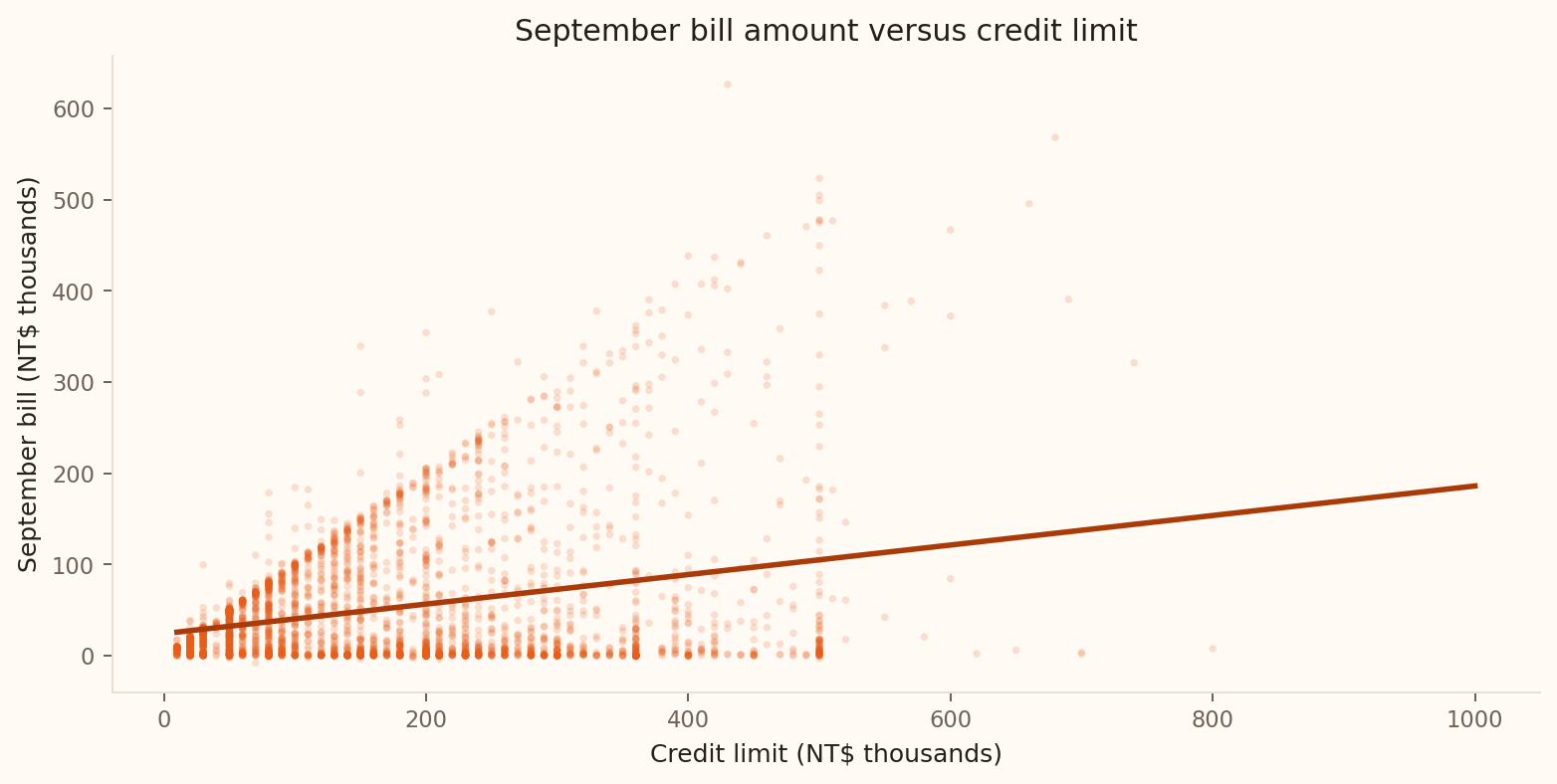
Scatterplots: two numerical variables
Allow three minutes. Each point represents a client: credit limit is on the horizontal axis and September bill amount on the vertical axis. Ask students to describe direction, form, strength and unusual observations from the picture. The fitted line shows the upward trend, while the spread around it remains substantial. Keep this discussion visual; correlation and regression are introduced in Week 8.
Chart guide: one variable
Categorical
How many records use each contact method?
Bar chart
Counts or proportions; zero baseline
Numerical
Where do balances cluster, and how long is the tail?
Histogram
Bin width; any omitted extremes
Numerical
What is the smooth shape of the balance distribution?
Density plot
Bandwidth; area represents proportion
Numerical
What are the typical balance and central spread?
Boxplot
Median, IQR, whiskers and outliers
Choose the question first , then the chart. Label the variable and its units.
Allow one minute for this guide and one for the next. Return to the opening Wooclap responses after students have seen the charts. Bars compare separate categories; histograms group numerical observations into intervals. A density curve smooths numerical data, while a boxplot gives a compact summary of location and variability. These are different views of a distribution, so the choice depends on the question. A boxplot alone can hide multiple peaks; the histogram and density examples illustrate what a five-number summary omits.
Chart guide: comparisons and change
Numerical + categorical
How do credit limits differ by default group?
Side-by-side boxplots or violins
Compare centre and spread; violins also show shape
Two categorical
Do subscription rates differ by contact method?
Mosaic plot
Width = group size; height = within-group proportion
Two numerical
Are credit limit and bill amount related?
Scatterplot
Direction, form, strength and unusual points
Numerical over time
How does review workload change each month?
Line chart
Time order, trends, spikes and gaps
Use the same units and scales for comparisons; make group sizes clear.
Allow one minute. Ask students to match each chart back to the example just shown. Boxplots compare quartiles and spread; violins add a smoothed view of the distribution, so their appearance depends on bandwidth. A mosaic shows both category-group sizes and conditional proportions. Grouped bars are another option for two categorical variables: decide whether the question concerns counts or within-group rates and label the denominator. Scatterplots concern paired numerical observations, whereas line charts use a meaningful order such as time. Week 8 develops the scatterplot example through correlation and regression.
Avoid chart decoration
Keep
Readable labels, units, source, honest scale
Remove
3D effects, heavy grids, redundant legends, clip art
The purpose of a chart is comparison, not decoration.
Allow one minute to summarise chart presentation. The preceding guides answer which chart to choose; this slide brings together how to present it clearly. Refer back to the bar chart’s zero baseline, the histogram’s labelled intervals, the line chart’s time order and the scatterplot’s labelled axes. Across the examples, keep the information needed to read the pattern: variables, units, source and an appropriate scale. Use this as a presentation check for the closing summary and dashboard activities.
Choose a useful summary
A small number of very large balances pull the mean above the median. Which would you lead with to describe a typical customer?
Mean alone
Median, supported by a distribution plot
Maximum balance alone
Correlation
Format: multiple choice, one answer. Allow 3 minutes total: 1 minute to vote, then 2 minutes for an explanation and debrief. Correct: option 2. The median resists extreme balances, while a plot and spread measure reveal what the centre omits. The mean still matters for totals and resource planning.
Build the risk dashboard
The recorded bank balances have mean €1,362, median €448, and maximum €102,127. Which summaries and plots would you report, and what would you check before treating negative balances as errors?
Format: open response. Allow 9 minutes to close Statistical Graphics: 4 minutes for pairs to draft their dashboard, 1 minute to submit, then 4 minutes to compare two responses and debrief. Ask each pair to justify a location measure, a spread measure and a plot, and state what they would investigate about negative balances. Expected: median and IQR for typical balance, mean for aggregate exposure, histogram or density for skew, and checks of variable definitions and source records before classifying negatives as errors. The dashboard consolidates descriptive summaries and chart choices before the probability section.
Explore before modelling
Validate
Types and ranges
Summarise
Centre and spread
Visualise
Shape and groups
Explain
Findings and limits
Use this as a brief recap before the final takeaway. Connect the workflow to the bank examples: check balance definitions, summarise centre and spread, inspect the plots, then explain findings and the assumptions needed to generalise.