Recall last week’s two-loan case
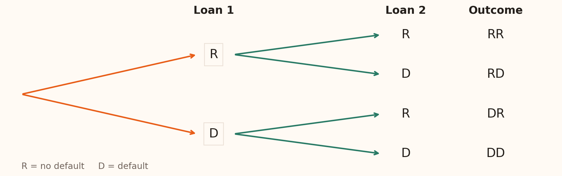
For two loans over the next year, \(S=\{RR,RD,DR,DD\}\) .
\(R\) means no default; \(D\) means default. Read the loans in order.
Which outcomes mean at least one default ?
If \(P(\text{no defaults})=0.81\) , what is \(P(\text{at least one})\) ?
Does listing four outcomes make each probability \(0.25\) ?
Five-minute opening retrieval. Answers: RD, DR, DD; 1−0.81=0.19; no, equal probabilities require a justified model. R denotes no default during the fixed horizon. This recalls the two-loan case from Session 2; the probability foundations are developed after counting.
Count the loan outcomes with a tree
\[2\times2=4\text{ outcomes: }RR,\ RD,\ DR,\ DD.\]
Counting rule: multiply the numbers of choices at successive steps: \(n_1n_2\cdots n_r\) .
Allow about seven minutes for this counting sequence, including the closing comparison table. Trace each path from Loan 1 to Loan 2. RD and DR are different outcomes because the loans are labelled. Each of the two first-loan branches has two possible second-loan outcomes, so there are 2×2=4 paths. In the general product rule, step i must offer n_i choices after every preceding path; the number may differ between steps. Counting does not require probabilistic independence or make the four paths equally likely. Revisit this same tree with branch probabilities after teaching multiplication and independence.
Combinations: count a selection once
Choose three distinct loan files from ten for audit.
A combination counts a selection once: \(\{A,B,C\}\) is the same set in any order.
Equivalent textbook notation (\(n\) available, \(r\) selected):
\[\binom{10}{3}=\frac{10!}{3!\,7!}=120.\]
\(n!=n(n-1)\cdots2\times1\) , with \(0!=1\) .
For 0≤r≤n distinct objects chosen without replacement, a combination records which objects are selected. Read the coefficient as “n choose r”. The five notations in the box all denote this same count; textbooks place the total and selected counts in different positions around C. The original lecture uses N for the total and n for the selection; here n and r retain the deck’s existing convention. Ask whether receiving A, B and C in a different order changes which files are audited. Define factorial before evaluating the formula: cancel 7! to get (10×9×8)/(3×2×1)=120. The r! denominator removes the repeated orderings of each selected set; the next slide makes those orderings explicit. Their probabilities depend on the selection mechanism. Session 4 will retrieve this notation when constructing count models.
Permutations: count each order
Now put the selected files into an audit queue . Order matters.
Each set of three files gives \(3!=6\) possible orders:
\[ABC,\ ACB,\ BAC,\ BCA,\ CAB,\ CBA.\]
Equivalent textbook notation (\(n\) available, \(r\) arranged):
\[\mathrm{P}(10,3)=3!\times120=10\times9\times8=720\text{ audit queues}.\]
The five notations shown in the original lecture all denote the same ordered count. A denotes arrangements and P denotes permutations; P(n,r) here is a count, while P(event) elsewhere denotes a probability. Multiply the 120 selections by the six orders per selection. Check the result with the product rule from the tree: ten choices for the first position, nine for the second and eight for the third. A permutation here uses distinct files without replacement, with 0≤r≤n. If repeated files were allowed, the three-position count would be 10³. Close by asking whether the task is to choose files or to schedule their order. Use the next comparison table to consolidate when each rule applies.
Choose a counting rule
Fill \(r\) positions from \(n\) options
Order matters; repeats allowed
\(n^r\)
Choose \(r\) objects from \(n\)
Order irrelevant; no repeats
\(\binom nr=n!/[r!(n-r)!]\)
Arrange \(r\) objects from \(n\)
Order matters; no repeats
\(n!/(n-r)!\)
For a multiple-step experiment with \(n_1,\ldots,n_r\) choices, use \(n_1\cdots n_r\) .
Count before assigning probabilities: equal counts imply equal probabilities only under an equally likely model.
Use this table to recap the tree, combination and permutation examples before introducing probability. Ask whether order matters and whether repetition is allowed. For example, four collateral grades and two review routes give 4×2=8 joint classifications if each grade allows both routes. Their frequencies need not be equal. For unequal numbers of available branches across earlier choices, count the possibilities for each branch and add.
Probability: what the number means
Probability is a numerical measure of the likelihood that an event or outcome will occur.
\(P(A)\) denotes the probability of event \(A\) .
\[0\le P(A)\le1,\qquad P(S)=1,\qquad P(\varnothing)=0.\]
\(0.1\) Unlikely: a 10% chance
\(0.5\) Equally likely to occur or not occur
\(0.9\) Likely: a 90% chance
The probabilities of all outcomes in a finite sample space sum to one .
This restores the original probability definition and scale. S denotes the sample space and the empty set denotes an impossible event. For our two loans, S={RR,RD,DR,DD}. The displayed probabilities are illustrative points on the scale, not fitted default rates. An impossible event has probability zero, but the reverse implication can fail for continuous outcomes; the exact review-time example appears in the closing distributions section. The next two slides explain two interpretations of the same mathematical probability rules.
Frequentist interpretation
Probability describes an event’s long-run relative frequency over comparable repetitions.
For a loan model with default probability \(p=0.02\) :
Observe many comparable loans over the same one-year horizon.
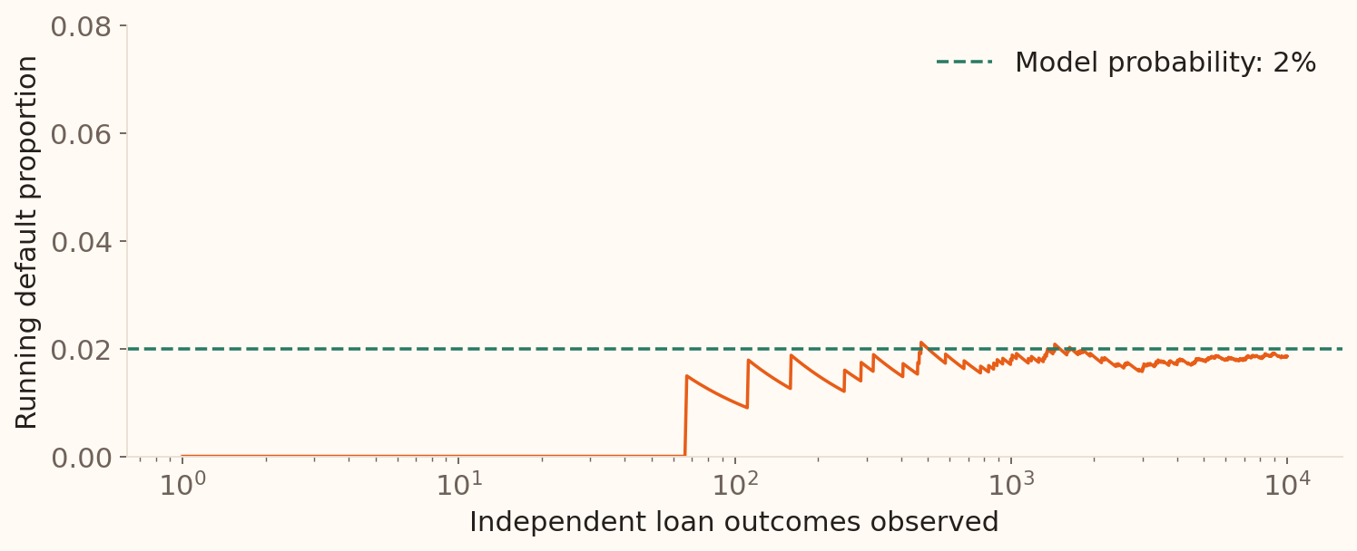
The proportion that default should be close to 2% in a sufficiently large collection under the model.
A small batch can contain zero, one, two or more defaults.
The underlying probability \(p\) is fixed; the observed proportion varies between samples.
The 0.02 probability is illustrative. Repeated observations refer to a stable process with the same event definition, population and observation horizon. The law of large numbers supplies the mathematical connection under conditions such as independent trials with a common probability. An observed default proportion estimates p; a finite sample does not reveal p exactly. Introduce the distinction between the model probability and an observed relative frequency before showing the simulation.
Bayesian interpretation
Probability expresses a degree of belief given the available information .
For the event “this loan defaults during the next year”:
Form a prior assessment using comparable loans and relevant knowledge.
Observe new evidence , such as repayment information.
Combine the prior and the evidence to obtain an updated probability .
Different information or model assumptions can lead to different assessments.
Both interpretations obey the same probability rules. Bayes’ rule will make the update precise later.
This restores the source’s degree-of-belief interpretation while making its basis in evidence explicit. A Bayesian assessment is conditional on stated information and assumptions; it is not an arbitrary number. Frequentist analyses also use conditional probabilities and update estimates with data. The distinction here concerns what probability means, including how uncertainty about unknown quantities is represented. Avoid presenting frequentist as “uses data” and Bayesian as “uses judgement”: both can use data, models and subject knowledge.
Law of large numbers: the long-run proportion
Observe independent trials with the same probability \(p\) of an event.
Here, independent means that learning one outcome leaves the other trials’ probabilities unchanged.
As \(n\) grows, the chance that \(\widehat p_n\) is close to \(p\) approaches one .
For loans with \(p=0.02\) , the running default proportion approaches 2% .
The hat distinguishes an observed estimate from the underlying model probability. “Close” means within any fixed positive tolerance: for every epsilon>0, P(|p-hat_n−p|<epsilon) tends to one. This is the weak law of large numbers for independent binary trials with a common p; independence and a common probability are sufficient conditions for this introductory version. Each observation has weight 1/n in the running proportion, so individual outcomes have less influence as n grows. A fixed finite sample can finish above or below p. Independence is introduced in words here and formalised after conditional probability.
Law of large numbers in the loan simulation
100
1
0.0100
1,000
18
0.0180
10,000
186
0.0186
Illustrative simulation: independent loans, \(p=0.02\) , seed 202603. The table gives points from the plotted sequence.
Compare the changing observed proportion with the fixed horizontal model line. Point out fluctuations in the curve as well as its overall stabilisation. The three table entries are checkpoints on this one simulated path, not three separate datasets and not a claim that every extra observation reduces the error. The 10,000-loan rate is close to 0.02 without equalling it. Session 4 will compare many fixed-size samples to explain sampling distributions and standard errors.
Does a quiet run change the next risk?
Assume independent loan outcomes with a constant 2% default probability. None of the first 50 loans defaults. What is the next loan’s default probability?
Less than 2%
Exactly 2%
More than 2%
50%
Allow 4 minutes including 60 seconds to vote. Correct: option 2. Calling the next default “due” is the gambler’s fallacy. Independence with a known, fixed p leaves the next probability at 2%. If p is unknown, a run can inform our estimate; if loans share an economic shock, the outcomes can be dependent. The next slide distinguishes the observed proportion from the next-loan risk and explains why the LLN requires no compensating run.
A quiet run and the next loan
Under the activity’s model, each independent loan has the same known risk \(p=0.02\) .
\[\widehat p_{50}=\frac{0}{50}=0,\qquad
P(\text{next loan defaults})=0.02.\]
A quiet run is possible; later loans keep the same risk.
The running proportion can fluctuate as it approaches \(p\) .
The LLN concerns a proportion over many trials . A finite batch can finish above or below \(p\) .
Calling a default “due” after a quiet run is the gambler’s fallacy .
The current observed rate and the model probability answer different questions. A long-run proportion can approach p without a compensating increase in the next-trial probability. Convergence does not promise exact equality at a finite n or a steadily decreasing error. The activity assumes p is already known and fixed. If p is unknown, observations can update its estimate; if a common economic shock links defaults, independence can fail. These distinctions connect the earlier interpretations to the probability assignments that follow.
Assigning probabilities
How do we choose a numerical probability for a defined event?
Classical Equally likely outcomes: favourable / total
Select one of 10 files uniformly; 3 are overdue, so \(P(\text{overdue})=3/10=0.3\)
Relative frequency Observed event count / observations
5,289 subscriptions in 45,211 campaign records give an observed rate of \(0.1170\)
Subjective Judgement informed by evidence and assumptions
Assess a new stress scenario using models, comparable cases and expert knowledge
State the event, observation period, evidence and assumptions behind the number.
This restores the three assignment methods from the original lecture after the LLN. Classical counting requires equally likely elementary outcomes. For historical frequencies, the LLN motivates estimation under stable, comparable sampling; a larger biased or changing sample need not represent the target process. The empirical campaign rate is 5289/45211=0.1169848, rounded to 0.1170. Applying it to a future customer requires a comparable population, campaign and observation horizon. Subjective assignments should state the evidence and assumptions and satisfy the probability rules. The methods describe how numbers are assigned; the frequentist and Bayesian slides describe how probabilities are interpreted.
From outcome probabilities to event probabilities
For \(S=\{RR,RD,DR,DD\}\) , use this illustrative joint probability assignment :
Probability
0.81
0.09
0.09
0.01
The probabilities sum to \(0.81+0.09+0.09+0.01=1\) .
Let \(A\) mean the first loan defaults and \(B\) the second loan defaults :
\[A=\{DR,DD\},\qquad B=\{RD,DD\}.\]
Add the probabilities of the outcomes in each event:
\[P(A)=0.09+0.01=0.1,\qquad P(B)=0.09+0.01=0.1.\]
This replaces the original oil-investment assignment with the existing two-loan example. The four values are a supplied illustrative joint distribution, not estimates from the cited datasets. They are nonnegative and sum to one. The probability of an event is the sum over its distinct outcomes in this finite sample space. That addition does not require independence. The later probability tree derives these same weights from independent loans with individual default probability 0.1. Keep the same A and B through complements, union, intersection and the addition rule.
Complement of an event
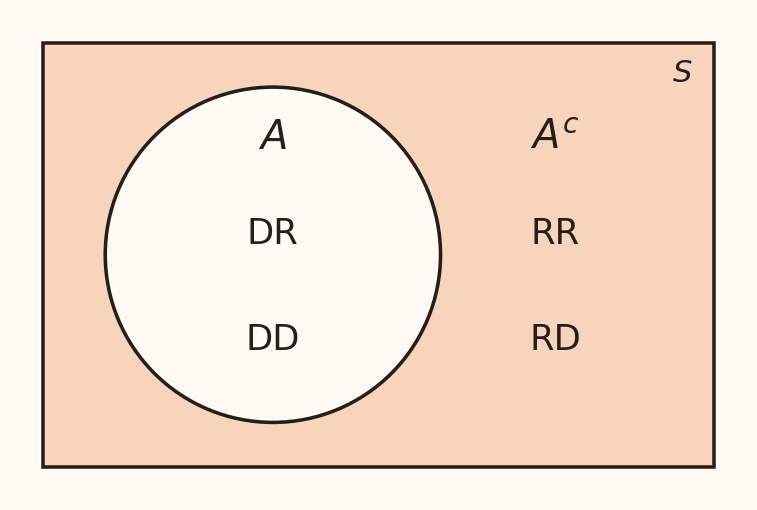
The complement of \(A\) contains all outcomes in \(S\) that are outside \(A\) .
Write it as \(A^c\) or \(A^{\complement}\) .
\(A^c\) : the first loan does not default .
\[A^c=\{RR,RD\}.\]
\[P(A^c)=1-P(A)=1-0.1=0.9.\]
Exactly one of \(A\) and \(A^c\) occurs, so their probabilities sum to one.
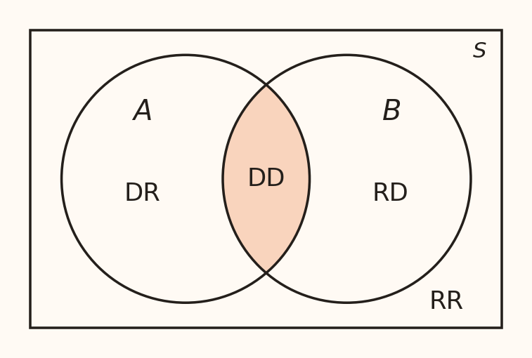
This restores a separate complement slide, including the complement notation used in the original TeX. Retrieve the two outcomes outside A from the diagram. The event and its complement are disjoint and together cover the sample space. The probability 0.9 also equals 0.81+0.09 from the supplied joint distribution. Diagram areas show membership, not probability size.
Union of two events
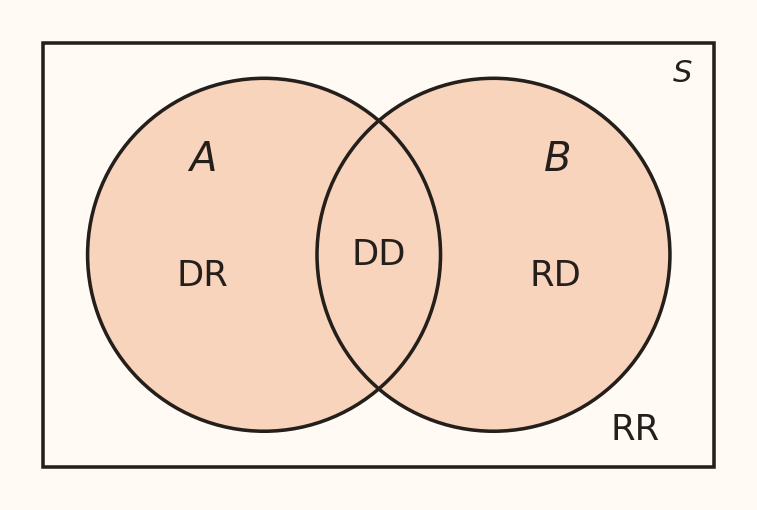
The union \(A\cup B\) contains outcomes in \(A\) or \(B\) , including outcomes in both.
\(A\) : first loan defaults; \(B\) : second loan defaults.
\(A\cup B\) : at least one loan defaults .
\[A\cup B=\{RD,DR,DD\}.\]
\[P(A\cup B)=0.09+0.09+0.01=0.19.\]
“Or” includes the possibility that both loans default.
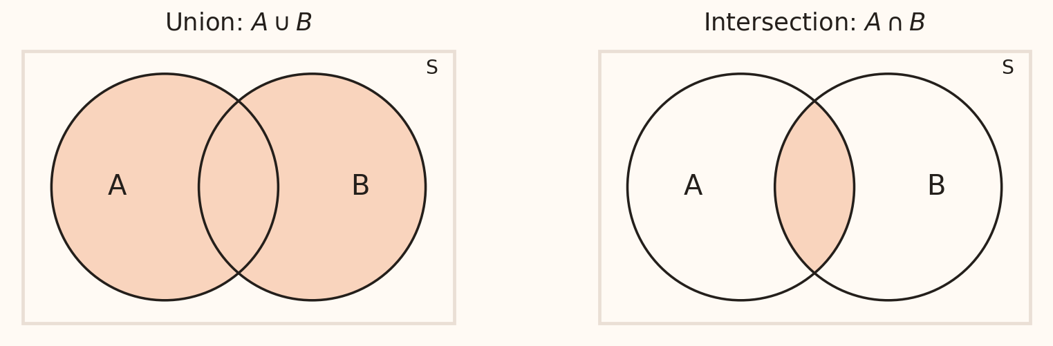
Trace the two circles and include their overlap once. RD and DR mean exactly one default; adding DD gives at least one default. RR is outside the union. This calculation directly adds the distinct outcome probabilities; the addition rule will soon provide the same answer from P(A), P(B) and their overlap.
Intersection of two events
The intersection \(A\cap B\) contains outcomes in both \(A\) and \(B\) .
\(A\) : first loan defaults; \(B\) : second loan defaults.
\(A\cap B\) : both loans default .
\[A\cap B=\{DD\}.\]
\[P(A\cap B)=P(DD)=0.01.\]
When we add \(P(A)\) and \(P(B)\) , how many times have we counted \(DD\) ?
Answer: twice. DD contributes 0.01 to P(A) and another 0.01 to P(B). A union should contain it once, motivating the subtraction on the next slide. The diagram shades only the intersection, correcting the original figure’s more ambiguous overlapping fills. No independence assumption is needed to read the supplied joint probability.
Addition rule
The overlap \(A\cap B\) was counted in both \(P(A)\) and \(P(B)\) , so subtract it once.
For our loans: \(P(A\cup B)=0.1+0.1-0.01=0.19\) .
Connect the preceding intersection slide’s shared outcome DD to the shaded intersection. The union includes the overlap once; adding P(A) and P(B) includes it twice. Develop the probability rule from that double count. The circles show set membership; their areas do not encode probabilities. For disjoint events the overlap is empty and the rule reduces to P(A)+P(B).
Two loan indicators in real data
Select a record uniformly from the 45,211 bank campaign records .
Let \(H\) mean housing loan and \(L\) mean personal loan.
\[P(H)=0.5558,\quad P(L)=0.1602,\quad P(H\cap L)=0.0966.\]
Use the exact counts to avoid rounding the intermediate values:
\[P(H\cup L)=\frac{25130+7244-4367}{45211}\approx0.6195.\]
About 62% have at least one of the two loan types.
Conditional probability
Conditioning changes the reference group from the whole sample space to event \(B\) .
Read \(P(A\mid B)\) as “the probability of \(A\) , given \(B\) ”.
The denominator is the probability of the information after the vertical bar. P(B)>0 is needed to define this ratio. Use the following table to show exactly which records remain in the reference group.
A two-way table
Let \(H\) mean housing loan and \(C\) mean campaign subscription.
No
3,354
16,727
20,081
Yes
1,935
23,195
25,130
Total 5,289 39,922 45,211
\[P(C\mid H)=\frac{1935}{25130}\approx0.0770,\qquad
P(H\mid C)=\frac{1935}{5289}\approx0.3659.\]
The same joint count, 1,935 , is divided by different reference groups.
Ask students to identify the row total for “given housing loan” and the column total for “given subscribed”. Read the results as 7.7% of housing-loan records subscribed, while 36.6% of subscriber records had a housing loan. The marginal subscription probability is 5289/45211=0.1170. These are probabilities for a uniformly chosen record from this dataset.
Multiplication rule
Rearrange the conditional-probability definition:
For the campaign table,
\[P(C\cap H)=\frac{1935}{25130}\times\frac{25130}{45211}
=\frac{1935}{45211}\approx0.0428.\]
Multiply a subgroup’s share by its conditional rate to obtain the joint probability.
Each conditional expression needs its conditioning event to have positive probability. Reversing the order gives the same answer: (1935/5289)(5289/45211). For three events, P(A∩B∩C)=P(A)P(B|A)P(C|A∩B). A tree records these conditional stages; independence is an extra condition, introduced next.
Independence
\(A\) and \(B\) are independent when knowing one does not change the probability of the other:
\[P(A\mid B)=P(A)\quad\text{when }P(B)>0.\]
Equivalently,
\[P(A\cap B)=P(A)P(B).\]
In the campaign records, \(P(C\mid H)=0.0770\) while \(P(C)=0.1170\) .
Housing-loan status and subscription are dependent in this empirical distribution.
The product definition is valid even if an event has probability zero. The exact joint probability is 1935/45211; it differs from (25130/45211)(5289/45211). The calculation describes association within the observed file. It does not estimate the effect of giving a customer a housing loan.
Mutually exclusive or independent?
Mutually exclusive Both cannot occur
\(P(A\cap B)=0\)
Independent Knowing one leaves the other’s probability unchanged
\(P(A\cap B)=P(A)P(B)\)
For one loan , default and no default are mutually exclusive.
For two independent loans , both can default: \(0.1\times0.1=0.01\) .
Two mutually exclusive events with positive probabilities are dependent.
If A has occurred and A and B are disjoint, B’s conditional probability is zero. This differs from its positive marginal probability. For distinct loans, independence is a modelling assumption; shared economic conditions can make their defaults dependent.
Add probabilities to the loan tree
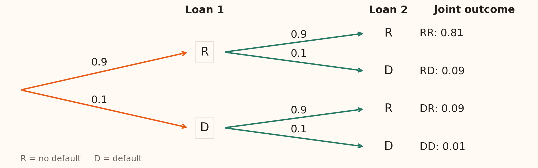
Multiply probabilities along a path; add probabilities across mutually exclusive paths.
\[P(\text{at least one default})=0.09+0.09+0.01=1-0.81=0.19.\]
Illustrative model: two independent loans, each with a 10% default probability.
Revisit the opening counting tree: the four outcomes are unchanged, and the model now supplies their probability weights. Independence makes the second-stage probabilities 0.9 and 0.1 on both branches; a tree can also represent dependence by changing those conditional probabilities. Each pair of outgoing branches sums to one, and the four joint probabilities sum to one.
Dependent events: sampling without replacement
An illustrative audit contains 10 files, 3 overdue . Select two files uniformly, without replacement.
Let \(O_1\) and \(O_2\) mean the first and second selected files are overdue.
\[P(O_1)=\frac3{10},\qquad P(O_2\mid O_1)=\frac2{9}.\]
\[P(O_1\cap O_2)=\frac3{10}\times\frac2{9}=\frac1{15}\approx0.0667.\]
Replacing and reshuffling the first file would give \(0.3\times0.3=0.09\) .
After an overdue file is removed, two overdue files remain among nine. If the first file is current, the second conditional probability is instead 3/9. The unconditional probability for the second draw is still 3/10: dependence concerns what we learn after observing the first draw. A fixed pool sampled without replacement does not give independent trials.
Total probability: split into two groups
Every occurrence of \(B\) lies either in \(A\) or in its complement \(A^c\) .
\[P(B)=P(B\cap A)+P(B\cap A^c).\]
Apply the multiplication rule to each part:
Overall probability = sum of each group’s share × its conditional probability.
Allow 12 minutes for this section: one for the rule, two for the problem, two for the diagram, three for the solution, two for the extension and two for the credit-data application. The groups A and A^c are disjoint and together include every application. Assume both have positive probability. Use A for the grouping event and B for approval throughout the paired total-probability and Bayes examples, matching the original lecture’s notation.
Loan approvals: the problem
A bank receives loan applications:
90% contain all required documents at submission.Of these complete applications, 95% are approved within one week.
Of applications with documents missing at submission, 30% are approved within one week.
Let \(A\) mean complete at submission and \(B\) mean approved within one week .
What is the probability that a randomly selected application is approved within one week, \(P(B)\) ?
Illustrative banking example; the probabilities are assumed.
This adapts the original assignment/exam problem and retains its inputs: P(A)=0.9, P(B|A)=0.95 and P(B|A^c)=0.3. Applications missing documents initially may supply them during the week. The outcome has a fixed one-week horizon. Ask students to identify the group shares and conditional probabilities before showing the diagram. The probabilities describe the illustrative model; they are not claims about a particular bank.
Loan approvals: draw the two routes
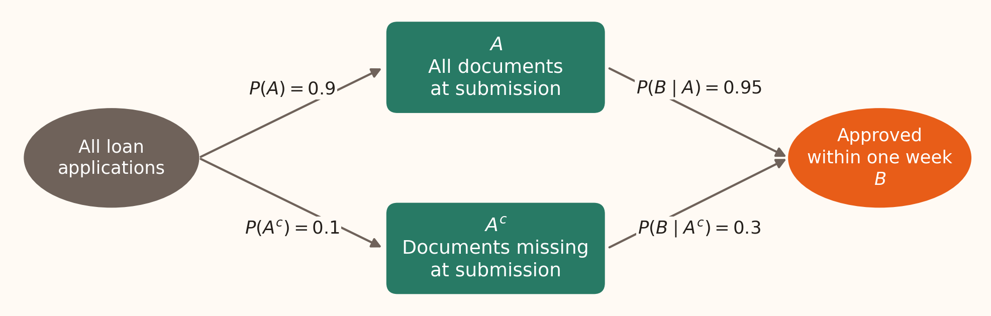
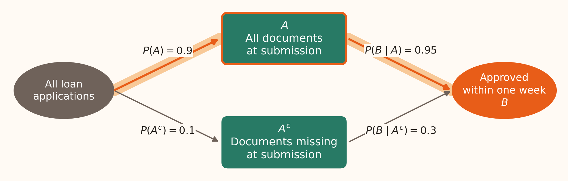
Multiply along each route to find its joint probability .
Add the two routes to include all approvals within one week .
The layout preserves the source diagram: all cases on the left, mutually exclusive groups in the middle, and one shared outcome on the right. The right-hand arrows show approval probabilities conditional on the middle groups. Non-approval outcomes are omitted because the question asks only about B; this is a diagram of the routes to B, not a full outcome tree. Arrow width and node area do not encode probability. Ask which number belongs to the lower first-stage arrow: P(A^c)=1−0.9=0.1.
Loan approvals: work through the solution
1. Split approval into disjoint events: \[B=(B\cap A)\cup(B\cap A^c).\]
2. Multiply along each route: \[\begin{aligned}
P(B\cap A)&=P(B\mid A)P(A)=0.95\times0.9=0.855,\\
P(B\cap A^c)&=P(B\mid A^c)P(A^c)=0.3\times0.1=0.03.
\end{aligned}\]
3. Add the joint probabilities: \[P(B)=0.855+0.03=\boxed{0.885}.\]
88.5% of applications are approved within one week in this model.
Have students calculate the two joint probabilities before revealing their sum. In an illustrative cohort of 1,000 applications, 900 begin complete and 100 begin incomplete. The model gives 855 approvals from the first group and 30 from the second, hence 885 overall. The simple average of 0.95 and 0.3 would weight unequal-sized groups equally. The total 0.885 lies between the two conditional rates and nearer 0.95 because the complete group is larger.
Total probability: extend to several groups
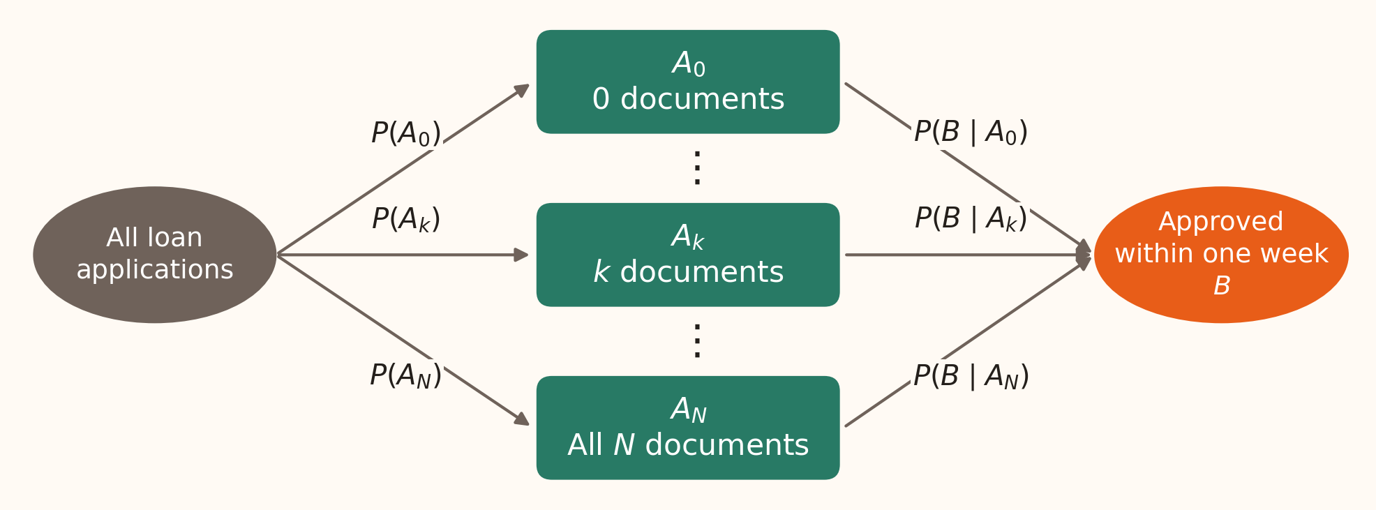
Suppose every application requires \(N\) documents. Let \(A_k\) mean exactly \(k\) were supplied at submission , for \(k=0,\ldots,N\) .
\[\begin{aligned}
P(B)&=P(B\mid A_0)P(A_0)+\cdots+P(B\mid A_k)P(A_k)+\cdots+P(B\mid A_N)P(A_N)\\
&=\sum_{i=0}^{N}P(B\mid A_i)P(A_i).
\end{aligned}\]
The groups form a partition : they cover all applications and do not overlap.
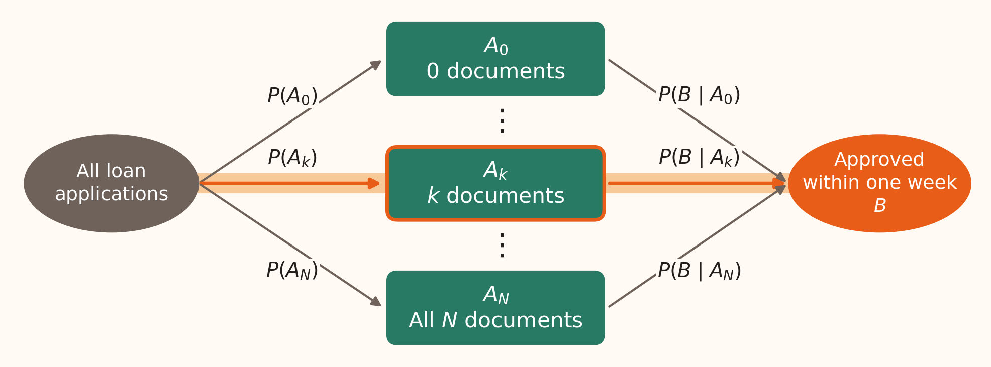
This restores the source’s A_0, …, A_k, …, A_N extension diagram, with document count replacing assignment count. Each application belongs to exactly one group, so their shares sum to one. Assume positive group probabilities when writing the conditional rates; omit any zero-probability groups. First read the diagram as a sum of P(B∩A_i), then apply the multiplication rule to each term. No independence assumption is required. The expanded sum includes the intermediate term P(B|A_k)P(A_k), highlighted when the same diagram returns for Bayes.
Real credit-default decomposition
No recorded delay
0.7727
0.1383
0.1069
One-month delay
0.1229
0.3395
0.0417
Two+ months delay
0.1043
0.6955
0.0726
For the first group, \(0.7727\times0.1383\approx0.1069\) .
Overall empirical default probability: \(0.1069+0.0417+0.0726=0.2212\) .
“No recorded delay” groups PAY_0<=0, “one-month delay” uses PAY_0=1, and “two+ months delay” uses PAY_0>=2. The shares and conditional rates are rounded. Calculate joint probabilities from unrounded counts, then add; rounding products displayed to four decimals can slightly change the final digit. The exact overall rate is 6636/30000=0.2212.
Bayes’ theorem: reverse the condition
Multiplication gives \(P(A\cap B)=P(B\mid A)P(A)=P(A\mid B)P(B)\) .
Therefore, when \(P(B)>0\) ,
\(P(A)\) \(P(B\mid A)\) \(P(A\mid B)\)
Bayes’ theorem updates the prior using evidence; total probability supplies the denominator .
Allow about 28 minutes for this section: two for the derivation, one for the loan question, one for its highlighted diagram, two for its solution, two for the extension, seven for the causal-reasoning comparison, one for the credit-flag setup, five for the activity and its two worked debriefs, and seven for base rates and discussion. Extend discussion as needed. This derives Bayes from the conditional-probability definition and multiplication. Prior means before using evidence B; posterior means after conditioning on B. The rule applies to empirical probabilities as well as models of beliefs. Reversing the condition does not establish a causal effect.
Loan approvals: reverse the question
Use the same bank and the same probabilities:
Complete at submission, \(P(A)\)
0.9
Approved within one week given complete, \(P(B\mid A)\)
0.95
Approved within one week given incomplete, \(P(B\mid A^c)\)
0.3
An application was approved within one week. What is the probability that it contained all required documents at submission, \(P(A\mid B)\) ?
Same illustrative model as the total-probability example.
The known event is now B. The question asks which initial group the application belonged to. Ask students to distinguish P(A|B) from the supplied P(B|A)=0.95. Total probability answered how often B occurs; Bayes asks how the B cases are distributed across the initial groups.
Loan approvals: highlight the required route
Numerator: approvals from the highlighted route through \(A\) .
Denominator: approvals from both routes to \(B\) .
This redraws the highlighted version of the source diagram. The arrows retain their forward direction because they show the supplied probabilities; Bayes uses these to answer the reverse question. Point to the entire highlighted route, not just its final conditional probability. The other route still belongs in the denominator. The posterior is a share of all approvals, not a share of all applications.
Loan approvals: work through Bayes
1. Find the highlighted joint probability: \[P(A\cap B)=P(B\mid A)P(A)=0.95\times0.9=0.855.\]
2. Include every route in the denominator: \[P(B)=0.855+0.03=0.885.\]
3. Divide the highlighted contribution by the total: \[P(A\mid B)=\frac{P(A\cap B)}{P(B)}
=\frac{0.855}{0.885}\approx\boxed{0.9661}.\]
Among applications approved within one week, about 96.6% were complete at submission.
Using the illustrative cohort from the earlier solution, 855 of the 885 approvals came from initially complete applications. The prior was 0.9; conditioning on approval changes it to approximately 0.9661. The complementary posterior is 30/885≈0.0339, and the two posterior probabilities sum to one. Do not confuse this result with the 0.95 approval rate among complete applications.
Bayes: extend to several groups
Given approval within one week, what is the probability that exactly \(k\) documents were supplied at submission?
\[P(A_k\mid B)=\frac{P(A_k\cap B)}{P(B)}
=\frac{P(B\mid A_k)P(A_k)}{\displaystyle\sum_{i=0}^{N}P(B\mid A_i)P(A_i)}.\]
One group’s contribution ÷ the sum of all groups’ contributions.
The document-count groups form the same partition as in the total-probability extension. Assume P(B)>0 and positive probabilities for the displayed groups. Trace the highlighted route through A_k for the numerator, then include every route for the denominator. Summing P(A_k|B) over k gives one. This extension belongs in the core lecture, as in the original .tex.
The same calculation applies to the three empirical credit groups on the preceding total-probability slide. For evidence D=default, P(two+ months late|D)≈0.6955×0.1043/0.2212≈0.328. Using exact counts gives 2177/6636≈0.3281. This reverses P(D|two+ months late)≈0.6955. The following flag exercise asks for that latter direction, using default and no default as its two initial groups.
Causality and Bayes’ Theorem
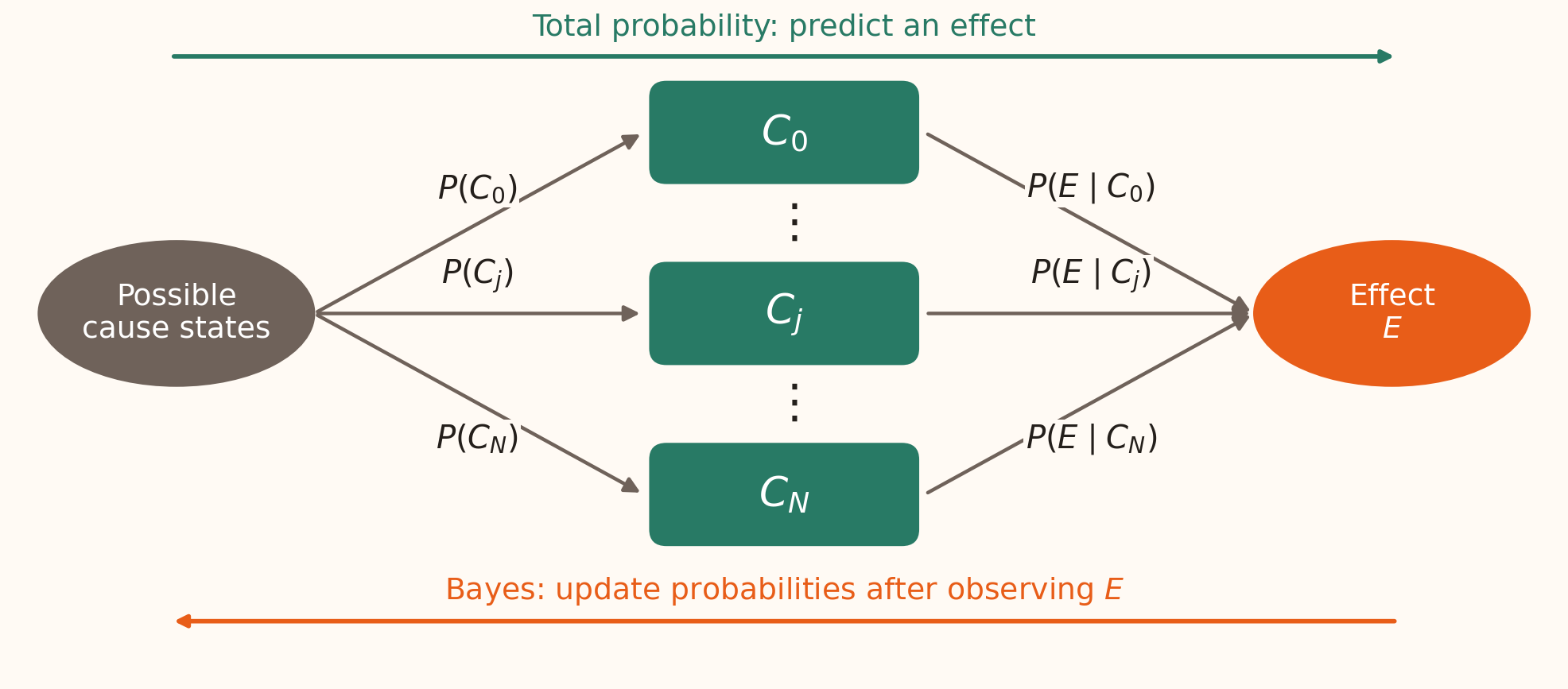
Under a causal model, let \(C_0,\ldots,C_N\) form a partition of possible cause states , and let \(E\) be the effect .
Predict: combine the routes to \(E\) . Diagnose: observe \(E\) , then update the probability of \(C_j\) .
Allow about seven minutes for these three causality slides. This redraws the original CauseEffect.PNG structure and makes the two directions of reasoning explicit. The C_i must be mutually exclusive and exhaustive states, with positive probabilities for the displayed conditional rates. Include a no-fault state and joint-fault states when faults can coexist; individual overlapping causes cannot simply be added.
For bank payments, a state could describe whether the network and internal processing system are working. A four-state partition is: neither fault, network fault only, internal fault only, and both faults. E is settlement after the promised deadline. A causal interpretation requires a justified mechanism; the probability identities also apply to groups that have no causal interpretation. The diagram organises the probability calculation and is not a causal discovery procedure.
Total probability vs Bayes: two directions
Total probability: predict
From possible causes to an effect
\[P(E)=\sum_{i=0}^{N}P(E\mid C_i)P(C_i).\]
Weight each state’s effect probability by how common that state is.
Banking question: across all system states, how likely is a payment to settle late?
Bayes’ theorem: diagnose
From an observed effect to a cause state
\[P(C_j\mid E)=
\frac{P(E\mid C_j)P(C_j)}
{\displaystyle\sum_{i=0}^{N}P(E\mid C_i)P(C_i)}.\]
Divide one state’s contribution by the total probability of the effect.
Banking question: a payment settled late; how likely is a network outage?
Total probability supplies the denominator that Bayes needs.
Use the same cause-state partition and conditional effect probabilities on both sides. Prediction averages over states before learning whether E occurred. Diagnosis conditions on E and updates the prior P(C_j) to P(C_j|E), assuming P(E)>0. If “network outage” includes several joint states, add their posterior probabilities. The inferred probability concerns whether the state occurred; attributing a particular payment’s delay to that state requires further causal assumptions.
Causal direction and direction of inference
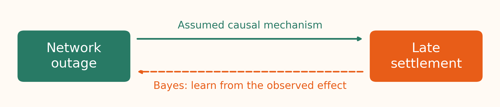
In an illustrative payment system, a network outage can delay settlement .
Observe a late payment: use Bayes to update the probability of an outage.Repair the network: ask how an intervention changes late-settlement probability.
Causal claims need a justified mechanism and study design. Bayes alone does not establish causation.
The physical direction in the assumed mechanism remains outage to delay. The backward arrow represents learning from evidence. Observing a delay changes our information; repairing the network changes the operating process. Conditional probabilities alone do not determine the effect of that intervention. Engineering knowledge, an appropriate experiment or explicit causal assumptions can support the causal model.
This also clarifies the earlier loan example: P(approval|complete documents) and P(complete documents|approval) describe different conditional groups. Estimating the effect of helping applicants complete their documents would require a causal comparison. Keep that distinction separate from the arithmetic of Bayes; no intervention notation is needed in this introductory lecture.
A simple arrears-review flag
Let \(D\) mean next-month default and \(F\) mean at least two months late in September.
Prior default probability, \(P(D)\)
0.2212
Flag given default, \(P(F\mid D)\)
0.3281
Flag given no default, \(P(F\mid D^c)\)
0.0408
Question: Among flagged accounts, what proportion defaulted, \(P(D\mid F)\) ?
Interpret the review flag
Given \(P(D)=0.2212\) , \(P(F\mid D)=0.3281\) and \(P(F\mid D^c)=0.0408\) , what is the probability of default given a flag , \(P(D\mid F)\) ?
7.26%
22.12%
32.81%
69.6%
Allow 5 minutes including this vote and the worked debrief on the next two slides. Give 90 seconds to calculate and vote. Correct: option 4. Ask for the full denominator before revealing the answer. Option 1 is the joint probability P(D∩F); option 2 is the prior; option 3 is P(F|D). All three are meaningful quantities, but only option 4 conditions on the flagged group.
Bayes calculation: combine both routes to a flag
\[P(F)=\underbrace{0.3281(0.2212)}_{\text{flagged defaults}}
+\underbrace{0.0408(0.7788)}_{\text{flagged non-defaults}}
\approx0.1043.\]
The flag updates the risk from 22.12% before conditioning to about 69.6% among flagged records .
Default and no default partition the sample space. Their prior probabilities are 0.2212 and 0.7788. Compute each joint probability before dividing by their sum: 0.07257572 and 0.03177504 using the rounded inputs. The resulting posterior is 0.6954978. The next table checks the same calculation using exact counts.
Check Bayes using the observed counts
Flagged
2,177
953
3,130
Not flagged
4,459
22,411
26,870
Total
6,636
23,364
30,000
\[P(D\mid F)=\frac{P(D\cap F)}{P(F)}=\frac{2177}{3130}\approx0.6955.\]
Finding: 69.6% of flagged records defaulted; 30.4% did not.
The numerator is 2177/30000 and the denominator is 3130/30000, so the full-dataset denominator cancels. A flag identifies a higher-risk subgroup in these historical records. Assess its performance on later data before making predictions for a new portfolio. The association does not show that flagging an account causes default.
Base-rate neglect: what is being neglected?
The base rate is the probability of default before using the flag , \(P(D)\) .
Base-rate neglect means judging a flag while ignoring how common defaults are in the portfolio.
In the credit data, a base rate of 22.12% led to about 69.6% default among flagged accounts .
Suppose only 2% of a new portfolio defaults, while the conditional flag rates stay the same. Would a flag still imply a 69.6% default probability?
Allow about seven minutes for this three-slide explanation. Define base rate before revisiting the numerical comparison. Here the error would be carrying the 69.6% posterior into a new portfolio without accounting for its lower default prevalence. Base-rate neglect means omitting or underweighting the prior; it can occur even when someone understands which conditional probability is being requested. Ask students to predict the direction of change before calculating.
See the base rate through account counts
Imagine 1,000,000 accounts , with a 2% default rate.
Keep \(P(F\mid D)=0.3281\) and \(P(F\mid D^c)=0.0408\) .
Default, \(D\)
20,000
32.81%
\(20{,}000\times0.3281=6{,}562\)
No default, \(D^c\)
980,000
4.08%
\(980{,}000\times0.0408=39{,}984\)
\[P(D\mid F)=\frac{6{,}562}{6{,}562+39{,}984}
=\frac{6{,}562}{46{,}546}\approx0.141.\]
The much larger non-default group contributes more flagged accounts , even with its lower flag rate.
Hypothetical portfolio; expected counts under the model, using the rounded UCI conditional flag rates.
These are expected counts, not observed records from a million-account dataset. The cohort size makes both products whole numbers and cancels in the ratio. Trace three steps: split accounts using the base rate; apply the appropriate flag rate to each group; divide flagged defaults by all flags. The exact calculation from these rounded rates gives 6562/46546≈0.1409788. Thus about 14.1% of flags are followed by default and 85.9% are not in this hypothetical model.
Same flag rates, different base rates
22.12%
32.81%
4.08%
About 69.6%
2%
32.81%
4.08%
About 14.1%
In the second portfolio, a flag still raises the probability from 2% to about 14.1% .
Most flagged accounts do not default , because non-defaulting accounts are much more common.
Interpret the evidence together with the portfolio’s base rate.
First row: UCI credit records, rounded rates. Second row: hypothetical portfolio with unchanged conditional flag rates.
For the hypothetical portfolio, 0.3281(0.02)/[0.3281(0.02)+0.0408(0.98)]=0.1409788. The flag remains informative: it multiplies the prior odds by the same likelihood ratio, 0.3281/0.0408≈8.04, in each row. Different starting odds therefore lead to different posterior probabilities. This odds explanation is optional; the count table supplies the main intuition.
Holding the conditional flag rates fixed isolates the role of the base rate. Those rates may also change in another portfolio; this comparison is a controlled hypothetical, not an estimate for a specific new bank. Ask students which two groups must appear in the denominator and what information was neglected when someone carried over the 69.6% figure.
From outcomes to numbers
A random variable assigns a number to each possible outcome.
Use uppercase \(X\) for the variable and lowercase \(x\) for a possible value: \(P(X=x)\) .
Discrete A finite or countably infinite set
Number of defaults: \(0,1,2,\ldots\)
Continuous Values over an interval
Time until an application is reviewed
Define what is measured, for whom, and over what period.
This restores the original notation and variable-type distinction before calculating moments. Discrete values need not be integers: a loss paid in fixed monetary increments is also discrete. Time can be modelled continuously even when recorded to the nearest minute. Arbitrary numerical codes for unordered categories do not acquire a meaningful mean just because they are numbers. The closing section develops PMFs and continuous densities; Session 4 applies these ideas to specific distribution families.
A random variable counts defaults
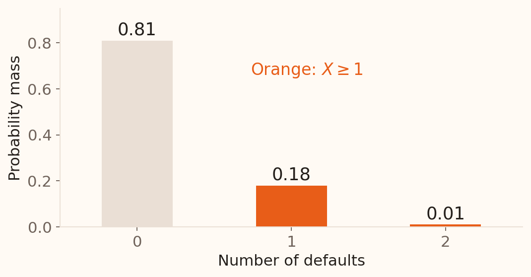
For two independent loans, each with default probability \(0.1\) , let \(X\) count defaults over the next year.
RR
0
0.81
RD or DR
1
0.18
DD
2
0.01
\[P(X=x)\ge0,\qquad \sum_xP(X=x)=1.\]
This table is the probability mass function (PMF) of \(X\) .
The original experiment has four outcomes, while X has three possible values. Add the probabilities of RD and DR because both map to X=1. A distribution can be described by a table, graph or equation. Its support is the set of values with positive probability. Check 0.81+0.18+0.01=1 before calculating moments.
Work out the expected loss
Two independent loans each have default probability \(0.1\) .
Probability
0.81
0.18
0.01
Each default causes an illustrative £1,000 loss .
Calculate the expected total loss. Can any one pair of loans lose exactly that amount?
Allow 4 minutes for paired calculation and discussion; the next slide provides the debrief. Expected defaults = 0.2, so expected loss = £200. The possible pair losses are £0, £1,000 and £2,000. £200 is the average loss over repeated pairs under this model. Ask why the mean alone does not describe loss risk, leading into variance.
Expected value
The expected value is the probability-weighted mean of the possible values.
\[E(X)=0(0.81)+1(0.18)+2(0.01)=0.20\text{ defaults}.\]
At £1,000 per default, expected total loss is £200 .
Week 2’s data mean weights each observed record equally; this distribution mean weights each possible value by its probability. In repeated independent pairs, the average count converges to 0.2 and the average loss to £200. An expected value need not itself be a possible outcome. For an infinite support, the expectation is defined when the relevant sum exists; all models used here have finite moments.
Variance of a random variable
Standard deviation is \(\sigma_X=\sqrt{\operatorname{Var}(X)}\) .
Variance averages the squared distance from the distribution mean .
SD expresses spread in the same units as \(X\) .
This uses the full specified probability distribution. The probabilities already supply the weights; there is no n−1 denominator. Week 2’s sample-variance formula estimates an unknown variance from observed data. The computational identity Var(X)=E(X²)−[E(X)]² gives a second way to check the next table.
Calculate the spread, one value at a time
For the default count, \(\mu=0.20\) .
0
0.81
0.04
0.0324
1
0.18
0.64
0.1152
2
0.01
3.24
0.0324
Total 1 0.1800
\[\operatorname{Var}(X)=0.18,\qquad SD(X)=\sqrt{0.18}\approx0.424\text{ defaults}.\]
Invite students to compute the final row’s contribution: a rare value can contribute substantially because its squared deviation is large. Check E(X²)=0²(0.81)+1²(0.18)+2²(0.01)=0.22, so Var(X)=0.22−0.20²=0.18. The variance has squared-count units. SD summarises spread; it is not a fixed interval containing a specified fraction of these discrete outcomes.
From counts to pounds
For constants \(a,b\) and \(Y=a+bX\) ,
\[E(Y)=a+bE(X),\qquad \operatorname{Var}(Y)=b^2\operatorname{Var}(X).\]
Here, total loss is \(L=1000X\) pounds.
Mean
0.20
£200
Variance
0.18
180,000 pounds squared
SD
0.424
£424.26
A fixed charge shifts the mean; scaling multiplies SD by \(|b|\) .
This brings the original Week 3 transformation context into the worked loss example. Var(1000X)=1000²(0.18), while SD(1000X)=1000√0.18=424.2641 pounds, using the unrounded count SD. Adding a fixed £50 administration cost makes the expected total £250 and leaves the SD at £424.26. These are illustrative loss amounts.
Combining losses
For random losses \(U,V\) and fixed weights \(a,b\) :
If the losses are independent ,
\[\operatorname{Var}(aU+bV)=a^2\operatorname{Var}(U)+b^2\operatorname{Var}(V).\]
Expected losses add even with dependence. The variance formula above needs independence.
Finite second moments are assumed. For dependent losses, add 2ab Cov(U,V); zero covariance is enough for the displayed variance rule, and independence guarantees it. For a difference U−V between independent quantities, the variance is Var(U)+Var(V), because the coefficient −1 is squared. Take the square root only after combining variances. Session 4 uses these rules to derive moments for specific probability models.
Two independent losses or twice the same loss?
Suppose \(U\) and \(V\) are independent, each with mean \(\mu\) and variance \(\sigma^2\) .
Two independent losses, \(U+V\)
\(2\mu\) \(2\sigma^2\)
Twice the same loss, \(2U\)
\(2\mu\) \(4\sigma^2\)
\(U+U=2U\) . Reusing the same random loss creates perfect dependence.
This corrects the original “X+X≠2X” slide. Algebra still applies: a nonconstant random variable is not independent of itself. As an optional numerical check, one loan’s loss is £0 with probability 0.9 and £1000 with probability 0.1, giving mean £100 and variance 90,000 pounds squared. Two independent such losses have variance 180,000 and SD £424.26; doubling one loss gives variance 360,000 and SD £600. The same expected £200 can therefore come with different variability.
Probability Distributions
Discrete probability distributions
A probability distribution describes how probability is allocated across a random variable’s possible values.
For discrete \(X\) , its probability mass function (PMF) is \[p(x)=P(X=x).\]
Possible values form a finite or countably infinite set.
Describe the same distribution using a table, graph or equation .
This restores the discrete-distribution recap at the original lecture’s ending, after moments and linear combinations. The source writes P(x); p(x) or f(x) are also used in textbooks for a discrete probability function. Always state that the function gives P(X=x). The sum runs over all possible values. The next slide revisits the two-loan table as an equation and graph, so no new probability model is needed.
Allow about 20 minutes for this closing distributions block, extending discussion as needed: four for the discrete recap and calculation; two for the continuous definition; eight for the histogram, density, interval and point sequence; four for the rectangle-area example; and two for the comparison.
Use a PMF to add probabilities
Let \(X\) count defaults among the same two independent loans , each with default probability \(0.1\) .
The earlier table can be written as \[p(x)=
\begin{cases}
0.81,&x=0,\\
0.18,&x=1,\\
0.01,&x=2,\\
0,&\text{otherwise}.
\end{cases}\]
\[P(X\ge1)=p(1)+p(2)=0.18+0.01=0.19.\]
Add the probability masses at the values belonging to the event.
Ask which bars belong to X≥1 before adding their heights. The table, equation and graph describe exactly the same distribution. PMF bar widths are a plotting choice: their heights give the probabilities. This prepares the contrast with a density, where interval area is the probability.
Continuous probability distributions
A continuous random variable can take values across an interval or collection of intervals .
We model it with a probability density function (PDF) , \(f(t)\) .
The probability of an interval is its area under the density : \[P(a<T<b)=\int_a^bf(t)\,dt.\]
This restores the original continuous-distribution introduction. Explain the integral as area; students need not evaluate an unfamiliar integral to read the following diagrams. A density’s height has units inverse to those of T, such as per minute. It is not the probability of a single value and can exceed one. A density need not be smooth; the flat density used later has jumps at its endpoints. We use continuous models with densities in this course.
A continuous example: loan-review times
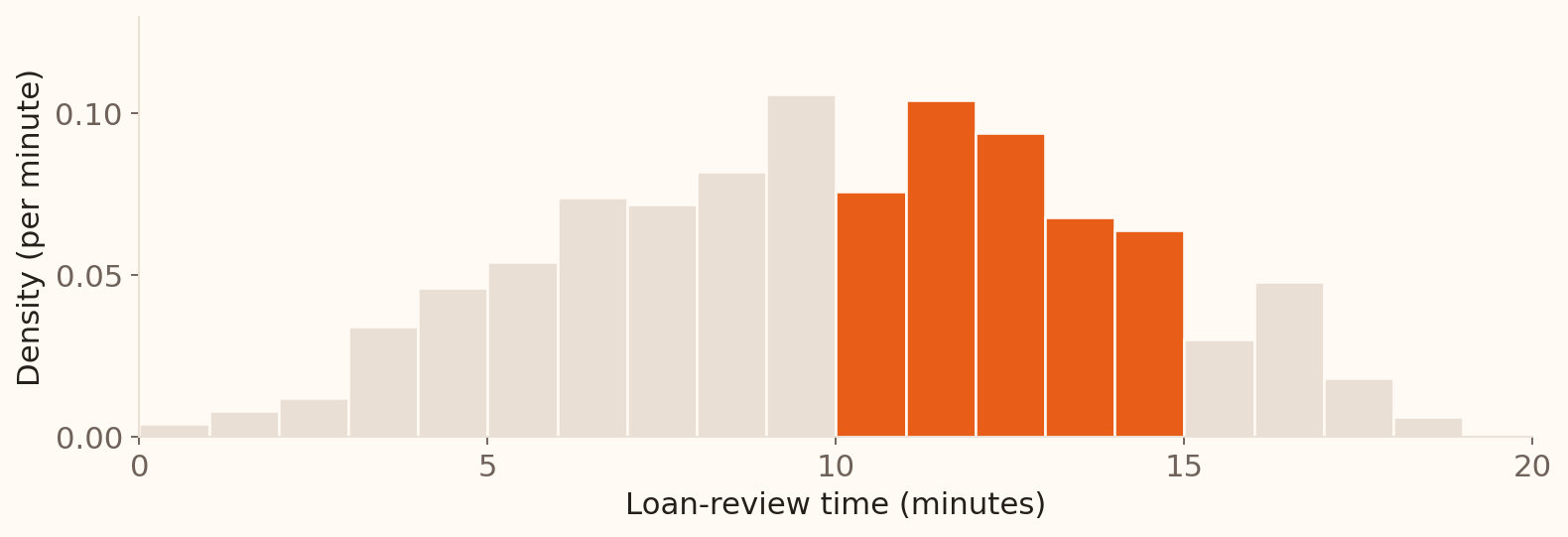
Let \(T\) be the time, in minutes, to review a loan application.
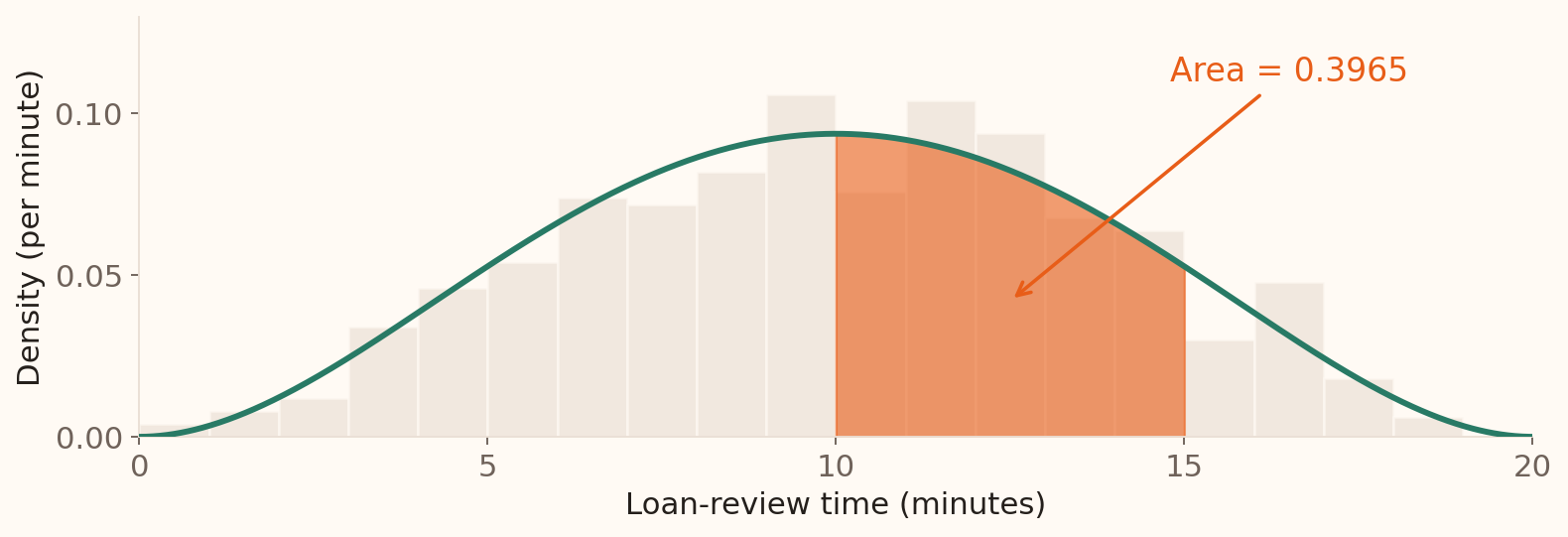
In this simulated sample, 203 of 500 reviews take between 10 and 15 minutes: \[\text{Sample proportion}=\frac{203}{500}=0.406.\]
Illustrative simulation of 500 review times; the histogram uses one-minute bins.
Ask students to identify the shaded bins before giving the proportion. The bins cover 10≤T<15. The histogram is scaled so each bar’s area equals its sample proportion; total area is one. Adding the highlighted bar areas gives 203/500. This is the observed proportion in one simulated sample; the probability supplied by its generating model follows on the next slides.
The simulation uses 20 times a Beta(3,3) variable, with NumPy seed 20261003. This family name is only for reproducibility; teaching here concerns the shape and area interpretation. The exact interval count and bin counts are recorded in verified-examples.json.
From a histogram to a continuous density
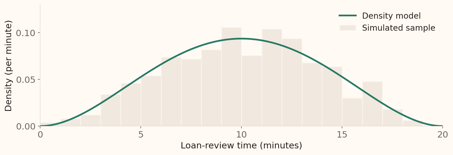
The histogram describes this sample. The density models how probability is distributed over review times.
Compare areas over intervals ; a new sample would give a different histogram.
Illustrative density model and one sample of 500 simulated review times.
This preserves the source’s histogram-to-density transition. The curve here is the known generating model, not a fitted curve or evidence from a bank. Sampling variation explains why the bars do not lie exactly on it. Model density and empirical histogram are distinct objects even though both have total area one. A smooth curve is useful in this example; smoothness is not a requirement for every density.
Probability is the shaded area
For the model, what is the probability of a review taking between 10 and 15 minutes ?
\[P(10<T<15)=\int_{10}^{15}f(t)\,dt\approx0.3965.\]
Model probability: about 39.65%. The sample proportion was 40.6% .
The interval probability is an area, not the height f(10), f(15), or the average of endpoint heights. The source’s shaded adult-height interval is replaced by a review-time interval, retaining the same graph sequence. For this supplied model, f(t)=30(t/20)2(1−t/20) 2/20 on 0≤t≤20 and zero elsewhere. Integrating gives 203/512=0.396484375. Students may take this curved area as supplied; the following flat-density example can be calculated geometrically. Endpoints have zero probability, so using ≤ instead of < leaves this probability unchanged.
An exact point has zero area
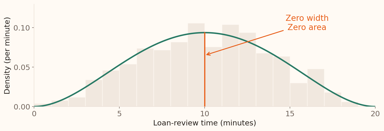
\[P(T=10)=0,\qquad\text{although }f(10)=0.09375.\]
Zero probability does not make an exact value impossible in a continuous model.
A recorded time of 10.0 minutes represents a rounding interval.
This restores the final point-probability diagram from the original lecture. The vertical line has height but no width, so its area is zero. It is possible to discuss P(T=t); that probability equals zero in this density model. Correct the source’s statement that it is not possible to talk about a particular value. The distinction is between zero probability and an empty event.
If a time is rounded to the nearest 0.1 minute, a displayed 10.0 represents approximately 9.95≤T<10.05. That interval has positive probability, about 0.0093748 under this model. Every single point has zero probability, while intervals contain uncountably many points; the positive interval probability does not contradict countable additivity.
A simple area calculation
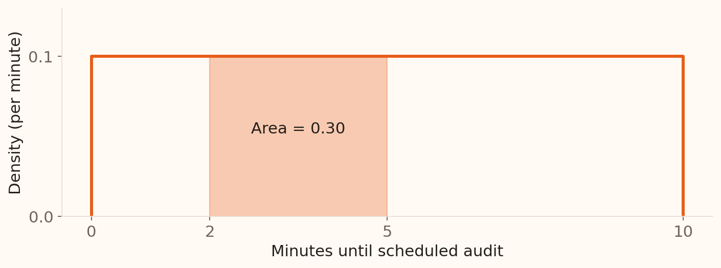
Suppose an audit starts at a time \(T\) chosen uniformly over the next 10 minutes .
\[P(2<T<5)=\underbrace{(5-2)}_{\text{width}}\times
\underbrace{0.1}_{\text{height}}=0.30.\]
Total area is \(10\times0.1=1\) .
This promotes the earlier reference preview into core teaching. The model and its parameters are illustrative. Have students calculate the rectangle area before showing the answer. Equal-length intervals have equal probabilities under this flat model. Session 4 names and develops the uniform family, including its mean and variance. An exact time still has zero probability, and adding or removing interval endpoints does not change the area.
Density height depends on units: expressing time in hours gives height 6 per hour over an interval of length 1/6 hour, with total area one. This demonstrates why a density may exceed one without violating probability rules.
Discrete and continuous: what carries probability?
Function
PMF: \(p(x)=P(X=x)\)
PDF: \(f(t)\)
Individual value
Can have positive probability
\(P(T=t)=0\)
Interval or event
Add the relevant probability masses
Find the area under the density
Total probability
\(\sum_xp(x)=1\) \(\int_{-\infty}^{\infty}f(t)\,dt=1\)
Banking example
Defaults among two loans
Time to review an application
A PMF gives probability at a value; a density gives probability through area.
Close by asking students whether a graph’s vertical value is a probability or a density. For a PMF it is a probability mass; for a PDF it is a density. Both distribute total probability one. The distinction concerns the model’s possible values, not simply whether a displayed number has a decimal point. A monetary amount restricted to fixed increments is discrete even when written with decimals.
Session 3 takeaway
The LLN connects a stable probability to the proportion observed over many trials.
Total probability combines group risks using the groups’ population shares.
Bayes’ rule updates a prior probability using new evidence and the base rate.
Expected value and variance describe the average and spread of a random loss.
Discrete probabilities add masses; continuous probabilities are areas under a density.
Next: choose models for individual outcomes, counts and waiting times, then explain why sample estimates vary.
Use the final 5 minutes for synthesis and questions. Ask students to distinguish the running default proportion from the next-loan risk, identify the weights in total probability and the denominator in P(D|F), and explain why an expected loss can be £200 when possible losses are £0, £1000 and £2000. Also ask students to contrast P(X=1) for a default count with P(T=10) for a continuous review time. These prompts connect the probability foundations, updating rules, random-loss calculations and distribution types.