Recall the two-loan model
Last week, each of two independent loans defaulted with probability \(0.1\) .
Let \(X\) count defaults over the next year.
\(P(X=x)\) \(0.81\) \(0.18\) \(0.01\)
What is the probability of at least one default?
How could we calculate these probabilities for 100 loans ?
A named probability model gives a reusable rule for a whole family of problems.
Retrieve P(X≥1)=1−0.81=0.19. The default probabilities are illustrative. Recall R for no default and D for default, with RD and DR distinct. Listing all 2^100 ordered outcomes would be cumbersome; the binomial model counts arrangements systematically. The model requires independent loans with a common default probability and the same observation horizon.
Begin with the question
One yes/no outcome
Does this loan default?
Bernoulli
Successes in a fixed number of trials
Defaults among 20 RBS loans
Binomial
Trials up to the first success
Monzo calls until a loan application
Geometric
Events in a fixed exposure
HSBC branch arrivals in one hour
Poisson
Define the variable and the observation window before choosing a formula.
This is a route map for the next block, not a memorisation test. Ask what is fixed: the number of trials, the stopping event, or the exposure time. The word success names the event coded 1; it can represent an adverse outcome such as default.
Bernoulli trial
One trial has two outcomes:
\[I=\begin{cases}1 & \text{success}\\0 & \text{failure}\end{cases},
\qquad P(I=1)=p,\quad P(I=0)=1-p.\]
\(p(1-p)\)
\(\operatorname{Var}(I)\)
\(\sqrt{p(1-p)}\)
\(SD(I)\)
For a loan, \(I=1\) can mean default . “Success” names the coded event.
This uses the Bernoulli introduction from the original Week 4 with a banking example. E(I)=0(1−p)+1p=p. Since I²=I, Var(I)=E(I²)−[E(I)]²=p−p²=p(1−p). I is an indicator; the count X on the next slide adds several indicators. The word success describes the value coded 1, regardless of whether the outcome is desirable.
RBS: how many loans will default?
Suppose Royal Bank of Scotland (RBS) has issued 20 loans , each with a 5% chance of default over the next year.
Let \(X\) count defaults: \(X=I_1+\cdots+I_{20}\) .
The binomial model assumes:
A fixed number of loans: \(n=20\) .
Two outcomes: default or no default.
The same default probability: \(p=0.05\) .
Independent outcomes across loans.
Thus \(X\sim\operatorname{Bin}(20,0.05)\) .
Illustrative RBS scenario: the portfolio size and default probability are teaching assumptions.
Define X in words before using the notation. The opening retrieval retains last week’s two-loan model with p=0.1; from here, the RBS example uses p=0.05 consistently. Independence means that learning one outcome leaves the other loans’ probabilities unchanged. A common economic shock or unequal borrower risks can challenge these assumptions. These are hypothetical parameters, not estimates from RBS data. First inspect four loans to see how arrangements work, then return to the full 20-loan portfolio.
Why a binomial probability counts arrangements
Let \(X\) count defaults among four of the RBS loans , each with default probability \(0.05\) . Exactly one default can occur in four disjoint ways :
1
DRRR
\(0.05(0.95)^3=0.04286875\)
2
RDRR
\(0.05(0.95)^3=0.04286875\)
3
RRDR
\(0.05(0.95)^3=0.04286875\)
4
RRRD
\(0.05(0.95)^3=0.04286875\)
\[P(X=1)=4(0.04286875)=0.171475.\]
Read the four loans in order; D means default and R means no default. This adapts the original Week 4’s four-person binomial derivation. Independence gives each path probability; constant p makes all four products equal; disjoint paths allow addition. Ask students to list the arrangements for exactly two defaults next. Introduce the combination formula after they have seen both examples.
Exactly two defaults: list every arrangement
For the same four loans, find \(P(X=2)\) . \(D\) = default; \(R\) = no default.
1 and 2
DDRR
\(0.05\times0.05\times0.95\times0.95=0.00225625\)
1 and 3
DRDR
\(0.05\times0.95\times0.05\times0.95=0.00225625\)
1 and 4
DRRD
\(0.05\times0.95\times0.95\times0.05=0.00225625\)
2 and 3
RDDR
\(0.95\times0.05\times0.05\times0.95=0.00225625\)
2 and 4
RDRD
\(0.95\times0.05\times0.95\times0.05=0.00225625\)
3 and 4
RRDD
\(0.95\times0.95\times0.05\times0.05=0.00225625\)
The six outcomes are disjoint, so add their probabilities :
\[P(X=2)=6\times0.00225625=\mathbf{0.0135375}.\]
Allow about two minutes. List pairs systematically: loan 1 with 2, 3 or 4; loan 2 with 3 or 4; and loan 3 with 4. This lists all six possible pairs once. For DDRR, multiply 0.05×0.05×0.95×0.95 using independence. Each other arrangement has the same product because it contains two defaults and two non-defaults with the same respective probabilities. Only one of these six ordered outcomes can occur, so their probabilities add: 0.00225625+0.00225625+0.00225625+0.00225625+0.00225625+0.00225625=0.0135375. Do not use the binomial formula yet. Ask students what the two examples have in common before generalising on the next slide.
From arrangements to the binomial formula
Both examples use number of arrangements × probability of one arrangement .
\(\binom nk\) Ways to place \(k\) successes among \(n\) trials
\(p^k\) Contribution of the \(k\) successes
\((1-p)^{n-k}\) Contribution of the \(n-k\) failures
For the six pairs we listed, \(\binom42=6\) .
Retrieve combinations from Session 3 after the concrete examples: choose which k of the n trial positions contain successes. There are n!/[k!(n−k)!] arrangements, and each has probability pk(1−p) (n−k). For the preceding two-default example, the coefficient counts the six listed pairs and the product is 0.00225625. The formula packages the counting, multiplication and addition students have already performed. At k=0 or k=n, the combination count is one, using 0!=1. The model’s support includes every integer from 0 to n when 0<p<1. The boundary cases p=0 and p=1 give certain counts of 0 and n respectively. Ask which part of the expression would be missed by calculating only one ordered path.
Binomial centre and spread
For \(X=I_1+\cdots+I_n\) , add the \(n\) Bernoulli means and, with independence, the \(n\) variances.
\(np\)
Expected successes
\(\sqrt{np(1-p)}\)
Standard deviation
For the 20 RBS loans with \(p=0.05\) , \(E(X)=1\) default and \(\operatorname{Var}(X)=0.95\) defaults².
Use the linear-combination rules from Session 3. The expectation of the sum is the sum of the expectations; the variance is the sum of variances because the trials are independent. Variances, rather than standard deviations, add. This connects the model-specific formulas to general probability tools students learned in Session 3.
Shape changes with \(p\)
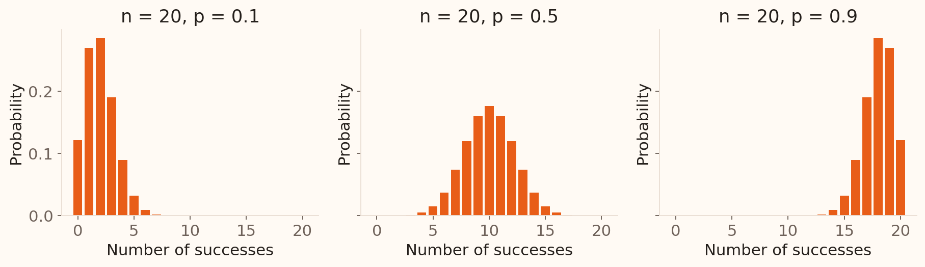
With fixed \(n\) , \(p\) changes the centre and shape. At \(p=0.5\) , the distribution is symmetric.
At fixed n, variance np(1−p) is largest at p=0.5. Small p places most mass near zero, leaving a right tail; p near one gives a left tail. Increasing n while holding 0<p<1 fixed reduces the standardised skew. This session introduces the normal model and the conditions for a normal approximation to binomial counts.
RBS: predict the default count
Return to the 20 independent RBS loans , each with annual default probability \(p=0.05\)
Define \(X\) and identify its distribution.
Find the expected number of defaults.
Find the chance of exactly two defaults.
Find the chance of at least one , using the complement.
Which model assumption would you check first in a real loan portfolio?
Illustrative RBS scenario; the same one-year horizon applies to every loan.
Allow 7 minutes including the worked debrief: 4 minutes calculating and 3 minutes comparing answers and assumptions. X counts defaults; Bin(20,0.05), E(X)=1, P(X=2)=0.1886768, P(X≥1)=1−0.95^20=0.6415141. Variance is 0.95 and SD is sqrt(0.95)=0.9747. Exactly two uses the binomial coefficient; at least one is quickest by complement. Discuss unequal borrower risks and shared economic shocks. The 5% probability is an illustrative model input.
RBS: work through the probabilities
Under \(X\sim\operatorname{Bin}(20,0.05)\) ,
\[E(X)=20(0.05)=1\text{ default}.\]
\[P(X=2)=\binom{20}{2}(0.05)^2(0.95)^{18}\approx0.1887.\]
\[P(X\ge1)=1-P(X=0)=1-(0.95)^{20}\approx0.6415.\]
Interpretation: about 18.9% of comparable 20-loan portfolios have exactly two defaults; about 64.2% have at least one under this model.
Illustrative RBS scenario: \(n=20\) , \(p=0.05\) , with defaults counted over one year.
Monzo: calls until a loan application
Monzo is a digital bank with no branches.
Suppose its call centre contacts potential customers to offer loans.
Each independent call has a 10% chance of prompting a loan application: \(p=0.1\) .
Let \(T\) count calls up to and including the first application .
Why geometric? Each call is a Bernoulli trial; we stop at the first success.
Illustrative calling scenario and 10% rate. Bank context: Monzo .
The call-centre scenario is hypothetical, not a description of Monzo’s current sales operations. A success means that the customer applies, not that the bank approves or issues a loan. Model comparable calls as independent with a constant p=0.1. Contrast the fixed 20-loan RBS portfolio with Monzo’s stopping rule: calls continue until the first application, so the number of calls varies. The photograph shows a Monzo card, consistent with its digital banking context.
Monzo: build the first few probabilities
Keep \(p=0.1\) . Let \(T\) count calls through the first loan application .
1
Applies
\(0.1\)
2
No, then applies
\(0.9(0.1)=0.09\)
3
No, no, then applies
\(0.9^2(0.1)=0.081\)
The number of calls varies because the stopping rule determines it.
Adapt the source’s first/third/tenth-trial progression to the Monzo example. With probability 0.9, a call produces no application; with probability 0.1, it produces an application. Multiply along the required sequence. The geometric convention includes the successful call, so possible values start at 1. If instead Monzo fixed the number of calls and counted applications, that count would be binomial under the same independent-trial assumptions.
Geometric probabilities: a long right tail
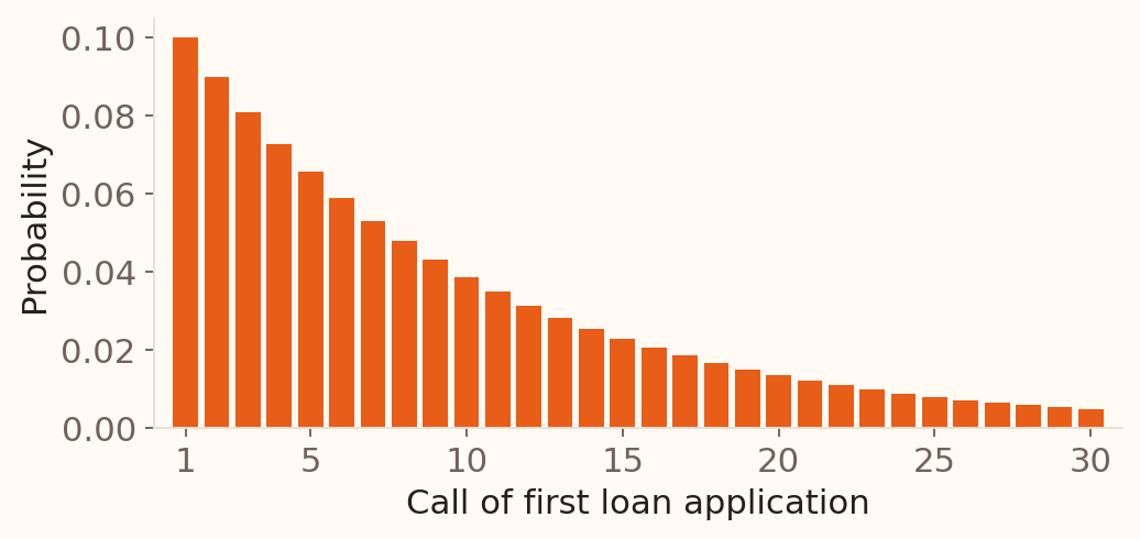
To finish on call \(k\) : first \(k-1\) calls fail, then one succeeds.
Call 1 is the most likely finishing point, but repeated failures can produce long waits .
After a failure, the next call still succeeds with probability \(p\) .
The plot shows the first 30 possible waits; the geometric distribution continues indefinitely. Connect the descending bars to the repeated factor 1−p in the PMF. The mode is 1, but the long right tail raises the mean above 1. For non-negative integers s and t, P(T>s+t | T>s)=P(T>t); independence and a constant p make the model memoryless. After any unsuccessful call, the remaining wait has the same distribution as a fresh wait. This restart idea motivates the next slide. Customer selection or learning can change the assumption in practice.
Why is the expected wait \(1/p\) ?
Let \(m=E(T)\) . For Monzo, \(p=0.1\) . Consider the first call :
Applies: stop
\(0.1\) \(1\)
Does not apply: start afresh
\(0.9\) \(1+m\)
The average combines these two possibilities:
\[m=0.1(1)+0.9(1+m)=1+0.9m.\]
So \(0.1m=1\) , giving \(m=10\) calls
Allow about two minutes. Every calling sequence uses one call. A successful first call adds no further wait; after a failure, independence and a constant success probability leave a fresh geometric wait with mean m. The 1+m in the table is the conditional average total wait after an initial failure, not a fixed number of calls. Weight the two conditional averages by their probabilities. The same unknown mean appears on both sides because the remaining process is unchanged.
As a long-run check, a success probability of 1/4 means about one success per four calls, hence an average spacing of four calls between successes. In general, a success rate p corresponds to an average spacing 1/p. The definition counts the successful call. An average over many calling sequences can be fractional even though each actual wait is an integer. The mean is neither a deadline nor the most likely wait. Finite mean follows from the geometric tail for 0<p≤1; p=0 would mean that success never occurs.
Variance: use the same first-call split
We know \(m=E(T)=1/p\) . Write \(v=\operatorname{Var}(T)=E[(T-m)^2]\) .
After a failure, \(T'\) is a fresh wait , with the same mean \(m\) and variance \(v\) .
Applies: stop
\(p\) \(1\) \((1-m)^2\)
Does not apply
\(1-p\) \(1+T'\) \(1+v\)
Both rows measure squared distance from the same overall mean \(m\) .
Why \(1+v\) ? Fresh deviations average zero; their squares average \(v\) :
\[E[(1+T'-m)^2]
=1+2\underbrace{E(T'-m)}_{0}+\underbrace{E[(T'-m)^2]}_{v}
=1+v.\]
Allow about two minutes. Retrieve Week 3’s definition: variance is the probability-weighted average squared distance from the overall distribution mean. The first-call split is exactly the one used for expectation. Success fixes T at 1. After failure, the total is one call already spent plus a fresh geometric wait T′. Independence and a constant p give T′ the same mean and variance as T.
Explain the final column before moving on. For success, the squared distance from m is (1−m)². After failure, the distance is 1+(T′−m). Expanding its square gives 1+2(T′−m)+(T′−m)². Fresh deviations average zero, while their squares average v, so the result is 1+v. Point to the two underbraces. This measures squared distance from the original mean m. Within the failure group, adding 1 shifts its mean to 1+m and preserves its variance v; the extra 1 comes from measuring distance to m. This distinction explains why averaging the conditional variances alone would miss a term.
Solve for variance, then SD
Weight the two rows by their probabilities:
\[v=p(1-m)^2+(1-p)(1+v).\]
Substitute \(m=1/p\) and collect the terms:
\[v=(1-p)v+\frac{(1-p)^2}{p}+(1-p)
=(1-p)v+\frac{1-p}{p}.\]
So \(pv=(1-p)/p\) . Divide by \(p\) to obtain variance; take its square root for SD.
For \(p=0.1\) : variance \(90\) calls²; SD \(\approx9.49\) calls .
Allow about two minutes. Average the squared deviations from the preceding table, using probabilities p and 1−p. Since 1−m=1−1/p=−(1−p)/p, the success contribution is p(1−m)²=(1−p)²/p. The terms outside v simplify as (1−p)²/p+(1−p)=[(1−p)²+p(1−p)]/p=(1−p)/p. Moving (1−p)v to the left leaves pv, giving v=(1−p)/p². Since p>0, sqrt(p²)=p, so SD=sqrt(1−p)/p. Every step follows from the first-call split and the definition of variance.
As a numerical check, take p=0.5 and m=2. The first-call table gives v=0.5(1−2)²+0.5(1+v)=1+0.5v, so v=2 and SD=sqrt(2)≈1.41. At p=0.25, mean=4, variance=12 and SD≈3.46. At p=1, every wait is exactly one and the variance is zero. In the Monzo example, SD≈9.49 is almost as large as the mean 10; the long right tail explains the large spread. Use p=0.1 throughout: variance=0.9/0.1²=90 and SD=sqrt(90)≈9.49. The distribution is right-skewed; mean ± SD is not a symmetric probability interval.
If a geometric variable counts only failures before the first success, its mean is (1−p)/p and its variance is unchanged. This deck consistently counts all calls through the success, with 0<p≤1.
HSBC: why model branch arrivals?
Suppose an HSBC branch receives an average of 10 customers per hour .
For the next hour , let \(X\) count customer arrivals.
The observation window is fixed; the count can be \(0,1,2,\ldots\)
How likely is a quiet hour with no arrivals ?
How likely are exactly two arrivals ?
To build a model, assume independent arrivals at a stable rate .
Illustrative HSBC scenario; 10 customers per hour is a model input.
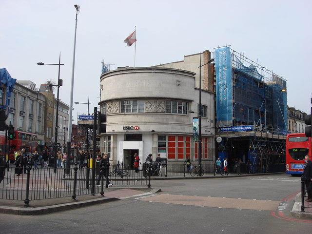
Allow two minutes. Start with branch staffing and workload before naming a probability formula. The clock determines when observation stops; the number of arrivals is random. Retrieve the contrast with RBS: 20 loans is a fixed number of trials, whereas HSBC’s hour is a fixed duration. An average of ten does not specify how often zero, two or many customers arrive. We will build a model using assumptions about short intervals, then answer these questions. Zero or two arrivals will be rare with this rate; use that as a reasonableness check. The photograph identifies the bank; the rate is hypothetical and is not measured at the photographed branch. Poisson models can also describe counts over fixed lengths or areas under analogous assumptions.
Build an hour from small time slots
Divide one hour into \(n\) equal slots. Approximate each slot by 0 or 1 arrival , independently, with a stable rate of 10 customers per hour.
Set the model’s arrival probability to \(p=10/n\) so that \(np=10\) :
100
36 seconds
0.1
10
1,000
3.6 seconds
0.01
10
10,000
0.36 seconds
0.001
10
Let \(I_j=1\) for an arrival in slot \(j\) , and \(0\) otherwise. The model count is
\[X_n=I_1+\cdots+I_n\sim\operatorname{Bin}(n,10/n).\]
Shorter slots improve this approximation when two or more arrivals in a very short slot are negligible.
Allow three minutes. The hour stays fixed while we refine its time grid; we are not extending the observation period. X_n is the constructed Bernoulli-slot approximation, while X is the count in the continuous-time arrival model. For n=100, E(X_n)=100×0.1=10. For n=1,000, 1,000×0.01 is still 10. The table probabilities are inputs to this approximation, not exact probabilities obtained merely from a stated average rate. Choose n large enough that 10/n≤1.
The homogeneous Poisson process assumptions are independent counts in disjoint intervals, a stable rate r, P(one arrival in a short interval of length Δt)=rΔt+o(Δt), and P(two or more arrivals)=o(Δt). Thus the total effect of slots with multiple arrivals vanishes as the grid is refined. The events can be common across a whole hour; it is their probability in each tiny slot that is small. Batch arrivals or shared shocks can violate the assumptions. If r is measured per hour and the observation lasts t hours, the same construction uses p=rt/n=λ/n.
Exactly two arrivals: start with binomial
Choose two arrival slots ; all the other slots must be empty:
\[P(X_n=2)=\binom{n}{2}\left(\frac{10}{n}\right)^2
\left(1-\frac{10}{n}\right)^{n-2}.\]
Choose the two slots and get their arrivals
\(\binom{n}{2}(10/n)^2=50(1-1/n)\to50\)
No arrivals in the remaining slots
\((1-10/n)^{n-2}\to e^{-10}\)
Multiply the limiting factors:
\[P(X=2)=\frac{10^2}{2!}e^{-10}\approx0.00227.\]
This limiting count model is the Poisson distribution .
Allow two minutes. This deliberately follows the earlier binomial arrangement explanation: choose which slots contain arrivals, multiply their arrival probabilities, and multiply the probabilities of empty slots. The combinations factor simplifies because n(n−1)/2 × 100/n² = 50(1−1/n). The next slide explains the empty-slot limit. At n=100, 1,000 and 10,000, the two-arrival probabilities are approximately 0.001623, 0.002200 and 0.002263, converging to 0.002270. These values are saved in the worked-example audit. The general-k algebra is in the notes on the general PMF slide. For k=0, the same empty-slot argument gives P(X=0)=e^−10, answering the quiet-hour question.
From two arrivals to the Poisson formula
For rate \(r\) over time \(t\) , write \(\lambda=rt\)
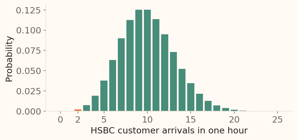
\[X\sim\operatorname{Pois}(\lambda):\qquad P(X=k)=e^{-\lambda}\frac{\lambda^k}{k!},\quad k=0,1,2,\ldots\]
For HSBC, one hour gives \(\lambda=10\) . The highlighted bar is \(P(X=2)\approx0.00227\)
Choose \(k\) slots and get arrivals:
\(\binom nk(\lambda/n)^k\longrightarrow\lambda^k/k!\) .
Keep the other \(n-k\) slots empty:
Each is empty with probability \(1-\lambda/n\) . Independence gives \(A_n=(1-\lambda/n)^{n-k}\) .
Use natural logs: \(\log(1-x)\approx-x\) for small \(x\) :
\(\log A_n\approx-(n-k)\lambda/n\longrightarrow-\lambda\) .
Exponentiating gives \(A_n\to e^{-\lambda}\) \(\lambda\) and \(k\) fixed as \(n\) grows.
Allow three minutes. Generalise the two-arrival example, explaining the empty-slot factor alongside the arrival-slot factor. With p=λ/n, the binomial probability for fixed k is C(n,k)(λ/n)k(1−λ/n) (n−k). The first part equals (λ^k/k!) times the product of (1−j/n) for j=0,…,k−1, so it tends to λ^k/k!. The empty-slot factor tends to e^−λ. Their product is the Poisson PMF. For k=0 use 0!=1, giving P(X=0)=e^−λ. The slot-selection factor includes both choosing the slots and obtaining an arrival in each. λ^k/k! alone is a probability weight and can exceed one; the product is the probability. The weights sum to e^λ, so the probabilities sum to one.
Distinguish rate r (customers per hour) from λ=rt (the expected number in the chosen window). The model count has no fixed upper bound. Here r=10 customers per hour and t=1 hour, giving λ=10. The definition of λ agrees with the binomial construction’s expected total; the next slide derives both moments.
A_n concerns a specified set of n−k slots. It is the empty-slot factor in the binomial calculation, not the entire probability of exactly k arrivals. Independent slots let us multiply their no-arrival probabilities. The chosen k slots are accounted for separately by the slot-selection and arrival factors. For k=0, A_n is the probability of no arrivals anywhere in the window.
Here log means the natural logarithm, the inverse of exp. Taking logs changes a product into a sum, making the accumulation of many small probabilities easier to see. Explain log(1−x)≈−x near x=0: for example, log(0.99)≈−0.01005, close to −0.01. The first-order expansion has error O(x²); after multiplication by n−k, the error is O(1/n) for fixed λ and k, so it vanishes. Since exp is continuous, log A_n→−λ implies A_n→exp(−λ). For λ=10 and k=2, the factor is (1−10/n)^(n−2), exactly the one on the preceding slide. The limiting value is about 0.000045400. Multiplying by the other limiting factor, 50, gives P(X=2)≈0.002270. Keep λ fixed because the observation window and its expected count stay the same as we refine the grid.
Why do mean and variance both equal \(\lambda\) ?
Reuse the binomial moments for the count from short slots, with \(p=\lambda/n\) :
\[E(X_n)=np=n\frac{\lambda}{n}=\lambda.\]
\[\operatorname{Var}(X_n)=np(1-p)
=\lambda\left(1-\frac{\lambda}{n}\right)\longrightarrow\lambda.\]
Each slot contributes \(p\) to the mean and \(p(1-p)\) to the variance. As \(p\) becomes tiny, these are almost equal; independence lets us add the variances .
For HSBC in one hour: mean 10 arrivals , variance 10 arrivals², and SD \(\sqrt{10}\approx3.16\) arrivals .
Allow three minutes. Connect to the binomial moment derivation and Week 3’s independent-sum rule. A Bernoulli slot has mean p and variance p(1−p); summing n slots gives np and np(1−p). The mean stays λ for every grid, while the variance approaches λ as the per-slot probability shrinks. For the one-hour model, the variances for 100, 1,000 and 10,000 slots are 9, 9.9 and 9.99, approaching 10. Their means are all 10. Explain the equal numerical values through many independent small contributions. Mean and variance have different units, so only their numerical values coincide for counts.
For an exact check from the Poisson PMF, E(X)=sum from k=1 of k e^−λ λ^k/k! = λ e^−λ sum from j=0 of λ^j/j! = λ. Likewise E[X(X−1)]=λ² by shifting the sum down by two, so E(X²)=λ²+λ and Var(X)=E(X²)−[E(X)]²=λ. These identities verify the limiting-moment rationale; convergence in distribution alone does not generally guarantee convergence of moments. For λ=0, X=0 with probability one and both moments are zero.
Equal-exposure counts from clustered arrivals or unequal rates can have variance above their mean. The Poisson equality is a property of this model; it is not a rule for every count dataset, and a finite sample mean and variance need not match exactly.
HSBC: rate and exposure
Keep the HSBC model: independent customer arrivals at 10 per hour .
30 minutes
5
\(e^{-5}\approx0.00674\)
1 hour
10
\(e^{-10}\approx4.54\times10^{-5}\)
2 hours
20
\(e^{-20}\approx2.06\times10^{-9}\)
In one hour, \(P(X\ge1)=1-e^{-10}\approx0.99995\) .
Doubling the window doubles the mean and variance ; SD increases by a factor of \(\sqrt2\) .
Illustrative HSBC model. Use the same time unit for rate and exposure; check for clustered arrivals and changing rates.
Allow two minutes. Revisit both questions from the opening slide: one hour has P(no arrivals)=e^−10≈0.0000454 and P(exactly two)≈0.002270. Across the three exposure windows, λ is 5, 10 and 20, with SD sqrt(λ). Counts over two disjoint one-hour windows add independently, so both their means and variances add. Pause for the ten-minute break here; resume with the model-choice activity to retrieve the four count/waiting models.
Choose the probability model
Match each question to Bernoulli, binomial, geometric or Poisson .
Is one transaction fraudulent?
How many of the 20 RBS loans default?
How many Monzo calls until the first loan application?
How many customers arrive at an HSBC branch in an hour?
Name one assumption needed for each choice.
Format: matching. Answers in order: Bernoulli, Binomial, Geometric, Poisson. Allow two minutes. Ask for common probability and independence for repeated trials, and stable rate and independent arrivals for Poisson. A single Bernoulli variable needs a defined binary outcome and its probability.
Model choice: explain what is fixed
One transaction: fraud or no fraud
Bernoulli
One defined binary outcome
Defaults among 20 RBS loans
Binomial
Independent trials with a common \(p\)
Monzo calls until the first application
Geometric
Independent trials with a constant \(p\)
HSBC arrivals during one hour
Poisson
Independent arrivals at a stable rate
Similar data can require different models when the question or stopping rule changes.
Use this after voting. For a single Bernoulli variable, no independence assumption is required; independence matters when combining trials. A fixed observation window alone does not establish a Poisson model, and a fixed portfolio size alone does not establish a binomial model. Ask which assumptions could fail when the customer mix or operating conditions change.
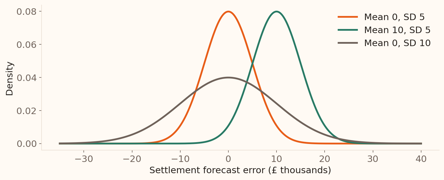
The normal family
\[X\sim N(\mu,\sigma^2)\]
Mean \(\mu\) sets the centre; SD \(\sigma\) sets the spread.
Illustrative models of settlement forecast errors, measured in £ thousands.
Read the normal model
\[X\sim N(\mu,\sigma^2)\qquad\text{means mean }\mu\text{ and variance }\sigma^2.\]
The curve is symmetric , with one peak at \(\mu\) .
Mean, median and mode all equal \(\mu\) .
The standard deviation is \(\sigma\) , in the same units as \(X\) .
Settlement forecast error: \(X\sim N(0,5^2)\) , measured in £ thousands .
Mean \(=0\) ; SD \(=5\) (£5,000); variance \(=25\) .
Compare the curves on the preceding slide. Throughout these slides, the second argument of N is the variance. This removes the source’s ambiguity between variance and SD parameterisations. The normal density is f(x)=exp(−(x−mu)²/(2sigma²))/(sigma sqrt(2pi)), for real x and sigma>0. It integrates to one. The normal family is also called Gaussian. The settlement-error parameters are illustrative; negative errors and positive errors are both meaningful.
Standardise: measure distance in SDs
Subtract the centre; divide by the standard deviation .
\(0\) \(0\) At the mean
\(10\) \(2\) Two SDs above the mean
\(-5\) \(-1\) One SD below the mean
Standardising preserves the event’s probability while changing its scale.
Use the same error model throughout the tail, interval and percentile examples. Emphasise the divisor 5, not 25. The z-score has no measurement units. A general variable can be standardised too, but standardisation alone does not make its distribution normal. Here normality is an explicit model assumption.
What does \(\Phi(z)\) tell us?
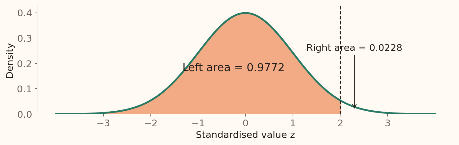
\(\Phi(z)=P(Z\le z)\) is the area to the left of \(z\) under \(N(0,1)\) .
\(\Phi(z)\) \(1-\Phi(z)\) \(\Phi(b)-\Phi(a)\)
A cumulative normal table or software gives \(\Phi(z)\) .
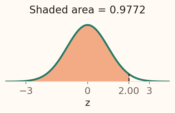
Introduce Phi before using it. A cumulative table gives area from minus infinity to z. Some tables instead show area from zero to z, so read the heading. For Phi(2.00), use row 2.0 and column 0.00 in a cumulative table to obtain 0.9772. The three table columns are the basic probability operations: read, complement and subtract. Symmetry gives Phi(−z)=1−Phi(z).
Read a standard normal cumulative table
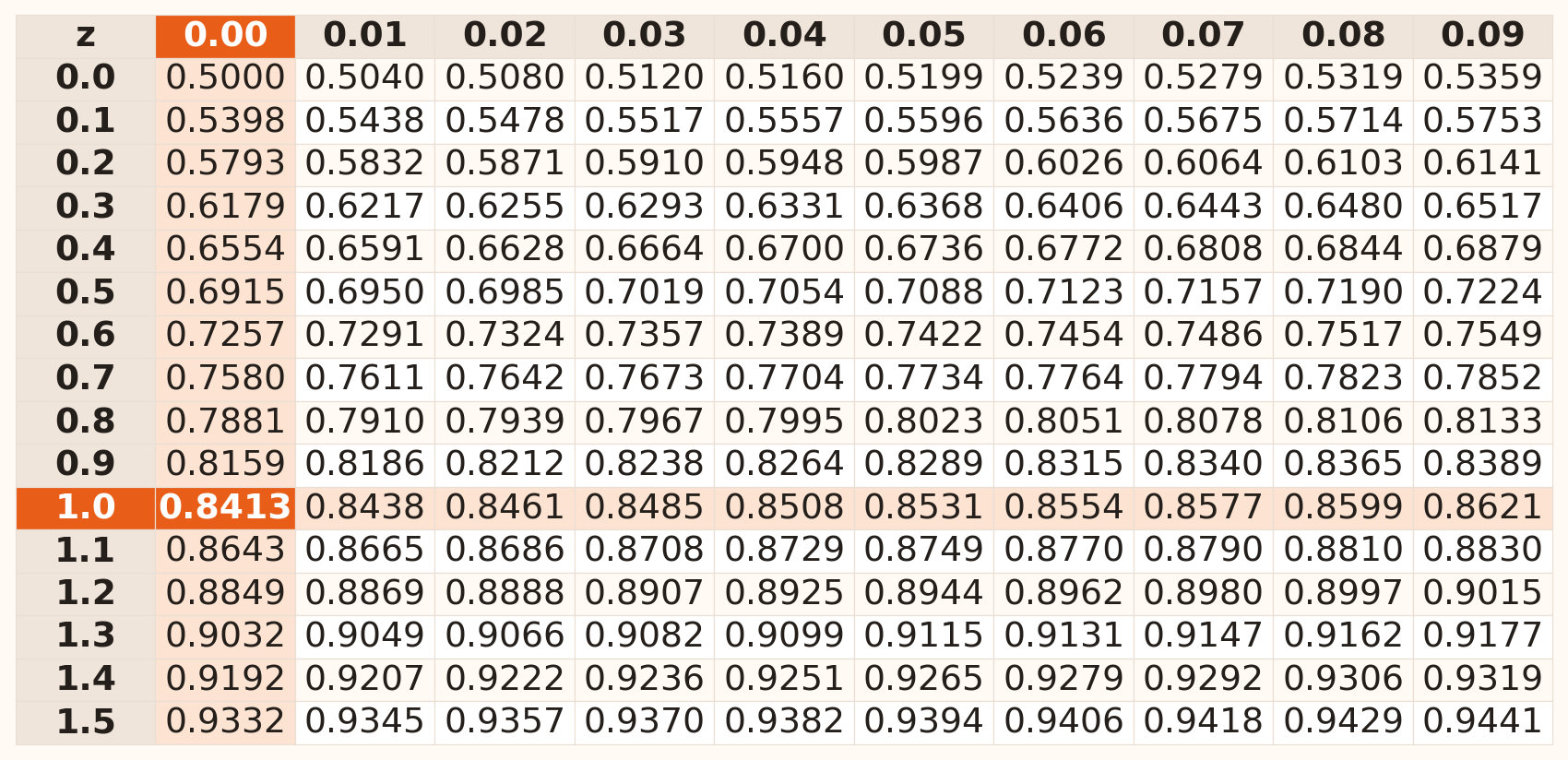
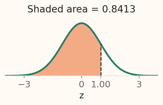
For \(Z\sim N(0,1)\) , each entry is \(\Phi(z)=P(Z\le z)\) \(z\) .
Read \(z=1.00\) :
Row 1.0 + column 0.00
\(\Phi(1.00)\approx\mathbf{0.8413}\) .
Symmetry:
\(\Phi(-1)=1-\Phi(1)\approx0.1587\) .
Table entries are rounded to four decimal places. Rows 0.0–1.5; the table continues on the next slide.
Allow about one minute. The table shows cumulative probabilities from minus infinity, matching the orange area. The row supplies the units and tenths of z; the column supplies the hundredths. Add the row and column labels to identify z, then read the probability at their intersection. Trace the highlighted row and column to 0.8413. Check that Phi(0)=0.5000 and that probabilities increase as z moves right. Negative z values follow from symmetry: Phi(−z)=1−Phi(z), so Phi(−1)≈0.1587. This retrieves the negative endpoint of the later settlement-error interval. Figures and all 310 table values are generated from the standard normal CDF by the course figure script.
Use the table for our \(z=2\) example
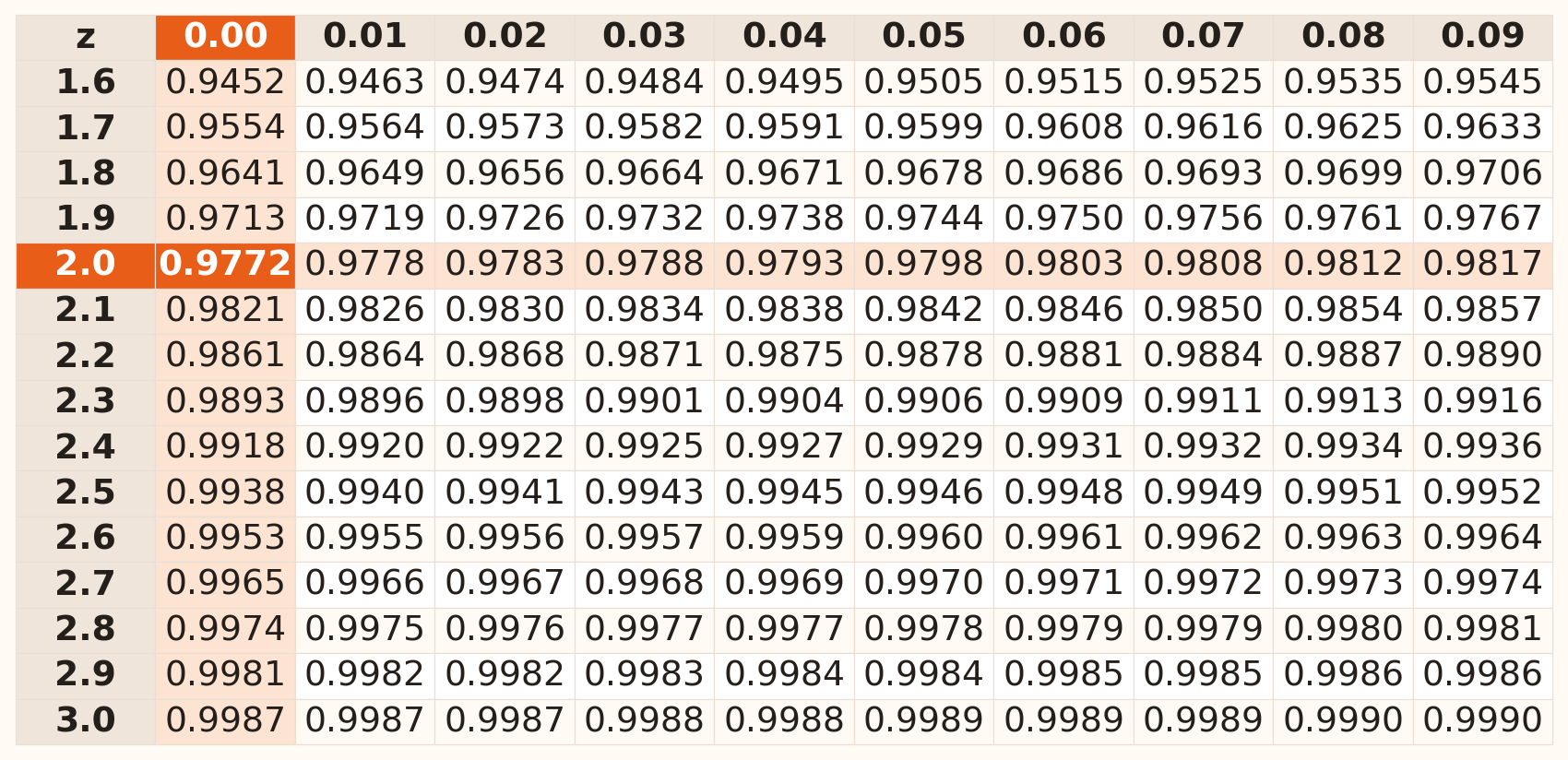
The same cumulative table continues below. Row + column gives \(z\) ; the cell gives \(\Phi(z)\) .
Read \(z=2.00\) :
Row 2.0 + column 0.00
\(\Phi(2.00)\approx\mathbf{0.9772}\) .
\(z=2.03\) :0.9788 in column 0.03 .
Table entries are rounded to four decimal places. For a right-tail question, subtract the table entry from 1.
Allow about one minute. Connect z=2.00 to the £10,000 threshold standardised using mean zero and SD £5,000. The row/column intersection gives the left area 0.9772; the following worked example takes its complement for the right-tail question. Ask students to find Phi(2.03) using row 2.0 and column 0.03, giving 0.9788. This distinguishes the tenths in the row from the hundredths in the column. For an additional percentile lookup, row 1.6 and columns 0.04 and 0.05 give 0.9495 and 0.9505, bracketing the later 95th percentile near 1.645. The interval example uses five-decimal software values; four-decimal table inputs give 0.9772−0.1587=0.8185 instead of 0.81859, a small rounding difference.
Forecast error: mark the event first
Suppose \(X\sim N(0,5^2)\) in £ thousands.
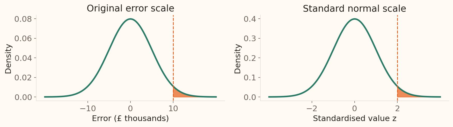
What is the chance that tomorrow’s forecast error exceeds £10,000 ?
Translate the question: \(P(X>10)\)
Allow students to identify the shaded tail and calculate z before showing the solution. Positive error is the model’s signed error measure; an absolute error above £10,000 would include both tails and would be a different question. The paired plots show that changing units changes the axis and density height, while preserving probability area.
Forecast error: calculate and interpret
Standardise the threshold: \(z=(10-0)/5=2\) .Read the left area: \(\Phi(2)=0.9772\) .Take the right tail:
Under the model, about 2.28% of days exceed this threshold.
Ask why 0.9772 is not the answer: the question asks for the area to the right. A percentage must refer to repeated comparable daily errors under this illustrative model. Keep full precision internally and round at the end. For a continuous model, P(X>10)=P(X≥10).
Interval probability: subtract two left areas
For the same model, what proportion of errors lies between −£5,000 and £10,000 ?
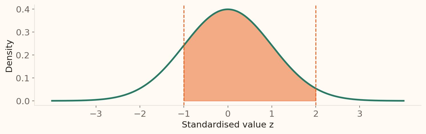
\[P(-5<X<10)=P(-1<Z<2)=\Phi(2)-\Phi(-1).\] \[\approx0.97725-0.15866=0.81859\approx\mathbf{81.86\%}.\]
Pause for students to standardise both endpoints before working the subtraction. Full precision gives 0.8185946. The displayed five-decimal inputs give 0.81859, preserving the final percentage when rounded. The interval need not be symmetric about the mean. It uses the same subtraction principle as the source’s quality-control example.
Percentile: work backwards from an area
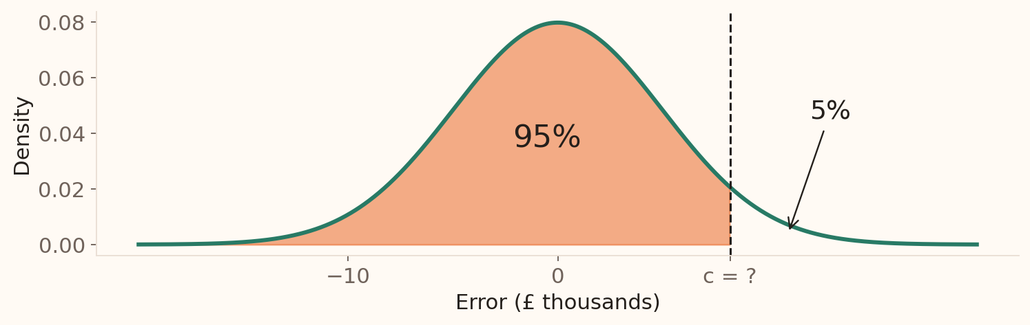
What threshold is exceeded on only 5% of days under the error model?
Find \(c\) such that \(P(X\le c)=0.95\) : the 95th percentile .
A probability question gives a threshold and asks for an area. This inverse question gives an area and asks for a threshold. First decide whether the 5% belongs in the left or right tail. Here it is the right tail, so the cumulative area is 0.95.
Percentile: return to the original units
Find the standard-normal percentile: \(z_{0.95}=1.64485\) .Undo standardisation: \(c=\mu+z_{0.95}\sigma\) .Substitute the error-model parameters:
The model places 95% below this threshold and 5% above it.
A table rounded to z=1.645 gives £8,225; software gives approximately £8,224.27. Either is consistent with its displayed precision. This is a percentile of individual daily errors. It is not a confidence limit for an unknown mean; sampling uncertainty comes next and confidence intervals are taught in Session 5.
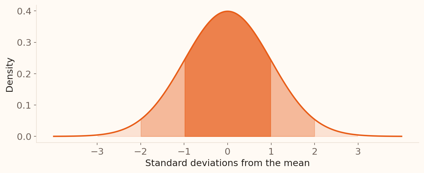
Three Sigma Rule
\(\mu\pm\sigma\) 68.27%
\(\mu\pm2\sigma\) 95.45%
\(\mu\pm3\sigma\) 99.73%
Barclays: why model balances on a log scale?
Suppose Barclays is analysing customers’ positive account balances .
In this scenario, most balances are modest; a few are very large. This produces a long right tail .
Let \(X\) be the balance in £ thousands , so \(X>0\) .
If \(\ln X\) is approximately normal, a log-normal model is a useful candidate for \(X\) .
Illustrative Barclays scenario. Zero balances and overdrafts need separate treatment.
The balance pattern is hypothetical, not a claim based on Barclays customer records. A right-skewed histogram motivates considering log-normality, but inspect the distribution of log balances before choosing the model. Restrict this example to positive balances because the logarithm is undefined at zero and is not real for negative balances. The photo provides bank context, not data for the model.
Barclays: the same balances on two scales
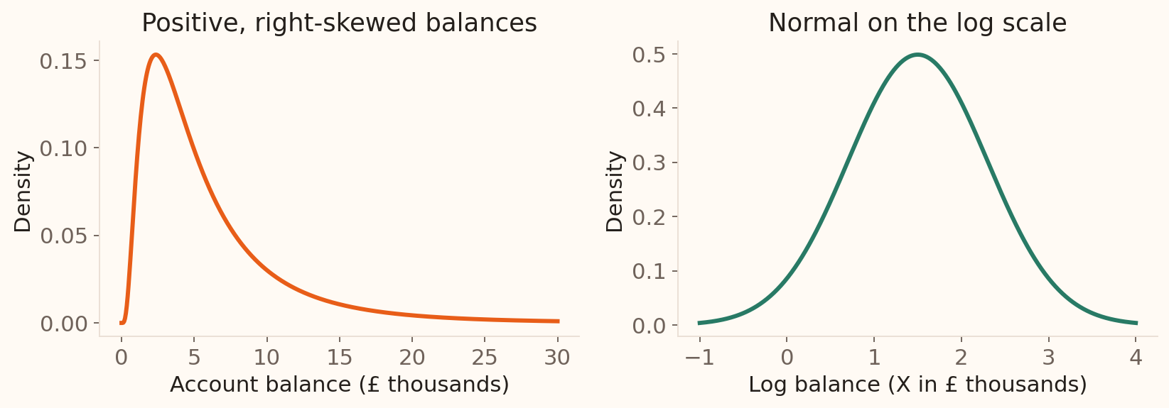
\(X\) is log-normal when \(\ln X\) is normal.
Taking logs compresses large balances. Check whether the logged values look normal.
Illustrative Barclays model: \(\ln X\) has mean 1.5 and SD 0.8; \(X\) is the balance in £ thousands.
Barclays: log parameters, mean and median
For the same balance \(X\) in £ thousands, suppose \(\ln X\sim N(1.5,0.8^2)\) .
Median balance
\(e^\mu\) \(e^{1.5}=4.48\)
Mean balance
\(e^{\mu+\sigma^2/2}\) \(e^{1.82}=6.17\)
The right tail pulls the mean (£6,172) above the median (£4,482) .
Multiplication becomes addition on the log scale: \(\ln(AB)=\ln A+\ln B\) .
Here mu=1.5 and sigma=0.8 describe the natural log of the numerical amount in the stated units. Neither is the mean or SD of the original amount. E(X)=6.171858 and median(X)=4.481689 in thousands of pounds. The variance is (exp(sigma²)−1) exp(2mu+sigma²), about 34.149 in squared thousands of pounds. The density is exp(−(ln x−mu)²/(2sigma²))/(x sigma sqrt(2pi)) for x>0, and zero otherwise. These supporting formulas belong here in the notes instead of in a later appendix. Positive multiplicative factors motivate a model on the log scale; inspect the log distribution to assess normality. Zeros need a separate part of the model.
Check the process, the shape and the decision
Binomial / geometric
Comparable trials, common \(p\) , independence
Poisson
Stable rate; counts and variability at the same exposure
Normal
Rough symmetry, one peak, plausible tails and range
Log-normal
Positive values; approximately normal natural logs
Check the part of the distribution that matters for the decision—especially a risk threshold or tail.
A model is a description of a process plus assumptions, not a label selected from shape alone. Compare equal exposures for Poisson means and variances. For a normal model, use a histogram and later a Q–Q plot; a good fit near the centre can coexist with poor tail probabilities. A hard boundary close to the centre or mixed subgroups can make a single normal model unsuitable. A skewed positive variable is a candidate for a log-normal model, but positivity alone does not establish that fit.
Poisson can approximate a rare-event count
Suppose 10,000 independent transactions each have fraud probability \(0.0003\) (0.03% ). Let \(X\) count fraudulent transactions.
Each transaction is a fraud / no-fraud trial , so the total count is binomial.
Many transactions + rare frauds reproduce our Poisson short-slot construction.
\[X\sim\operatorname{Bin}(10{,}000,0.0003),\qquad \lambda=E(X)=np=3.\]
For large \(n\) and small \(p\) , use \(Y\sim\operatorname{Pois}(3)\) : 3 expected frauds per batch .
Exact binomial: \((1-0.0003)^{10{,}000}\)
\(0.04976\)
Poisson approximation: \(e^{-3}\)
\(0.04979\)
Each transaction contributes an indicator: 1 if fraudulent and 0 otherwise. Adding these independent indicators with the same fraud probability gives the binomial count. Retrieve the earlier construction from short time slots, now applying it to many actual transactions. Because fraud is rare, the count is usually small even though there are many transactions; lambda=np=3 sets the scale of that count. The limiting argument has n growing, p shrinking and np held fixed. Here lambda is the expected total count, not a per-transaction probability. The exact binomial remains available in software. A Poisson arrival model and a Poisson approximation to fixed Bernoulli trials are related but distinct justifications. All numbers are illustrative, and independence can fail under organised or clustered fraud.
When can a normal curve approximate counts?
Suppose RBS receives 245 independent loan applications , each with a 25% chance of needing manual review . Let \(X\) count these reviews.
Many independent review/no-review outcomes can add up to a bell-shaped count .
Manual reviews: \(np\)
\(245\times0.25=61.25\ge10\)
No manual review: \(n(1-p)\)
\(245\times0.75=183.75\ge10\)
Match the binomial mean and variance:
\[Y\sim N\!\left(np,\ np(1-p)\right)=N(61.25,\ 45.9375).\]
Earlier fraud example: \(np=3<10\) ; it fails this check despite having 10,000 trials.
This illustrative RBS manual-review scenario retains the source’s n=245 and p=0.25. The outcome is whether an application needs manual review; this 25% probability is separate from the earlier 5% loan-default probability. Assume independent applications and a common review probability. Each review indicator is 0 or 1, and their sum X is Bin(245,0.25). Many small independent contributions motivate a bell-shaped approximation; requiring enough expected outcomes of both types helps avoid a count piled up near zero or n. Here np=61.25 and n(1-p)=183.75 both exceed 10. Match mean 61.25 and variance 45.9375, giving SD=sqrt(45.9375)=6.7777 reviews. The expected counts need not be integers, even though an observed count is always an integer. The expected-success and expected-failure checks are heuristics; they do not guarantee relative accuracy in extreme tails. In the previous fraud example, n=10,000 is large but np=3 fails this normal-approximation check; retain the binomial or its Poisson approximation. A large-mean Poisson count can also be approximated by N(lambda,lambda): a sufficiently large lambda reduces skew, but there is no universal cutoff for every event probability. Both approximations replace a discrete count by a continuous area, requiring the boundary adjustment shown next. These formulas use variance as the second normal parameter.
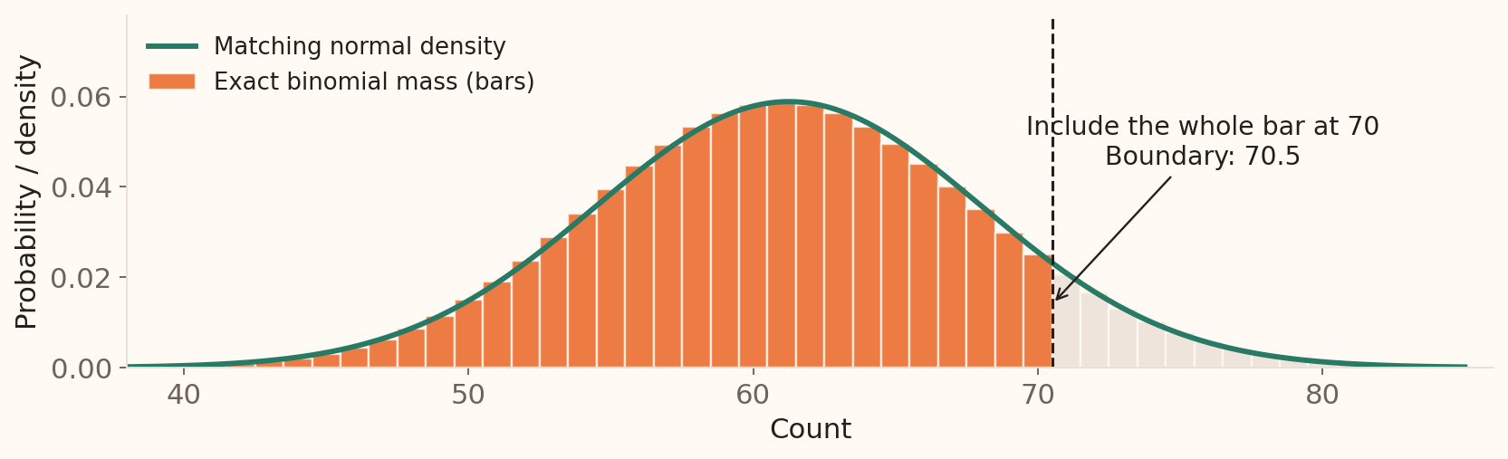
Continuity correction: give each count its width
\(X\le70\) \(Y<70.5\)
\(X\ge70\) \(Y>69.5\)
\(X=70\) \(69.5<Y<70.5\)
Here \(X\) counts RBS manual reviews ; each bar has width one .
The correction is geometric: each bar centred at integer k extends from k−0.5 to k+0.5. For an inclusive interval a≤X≤b, use a−0.5<Y<b+0.5. For X>70, the first included count is 71, so use Y>70.5. Continuity correction can improve both interval and tail approximations; it does not repair an unsuitable normal shape. The plot displays the central count range for readability.
Compare the approximation with the exact answer
RBS can handle 70 manual reviews among the 245 applications. For \(X\sim\operatorname{Bin}(245,0.25)\) , find \(P(X\le70)\) .
\[z=\frac{70.5-61.25}{\sqrt{45.9375}}=1.3648.\]
Exact binomial CDF
\(0.9123\)
Normal, boundary at \(70\)
\(0.9016\)
Normal, corrected boundary at \(70.5\)
\(0.9138\)
The corrected estimate is 91.38% that 70 review slots are enough.
Continue the illustrative RBS manual-review scenario: the bank has capacity to review 70 of the 245 applications, so capacity is sufficient when X<=70. Retain the source’s exact-versus-normal comparison, now with a worked continuity correction and unrounded SD. The corrected boundary includes the full probability bar for exactly 70 reviews. The exact probability is stats.binom.cdf(70,245,0.25); the corrected approximation is stats.norm.cdf(70.5,loc=61.25,scale=sqrt(45.9375)). This gives 91.38%, compared with the exact 91.23%. Exact functions are useful for checking approximation accuracy. The values in this table are independently audited by the Week 4 figure generator.
Relationships among common distributions
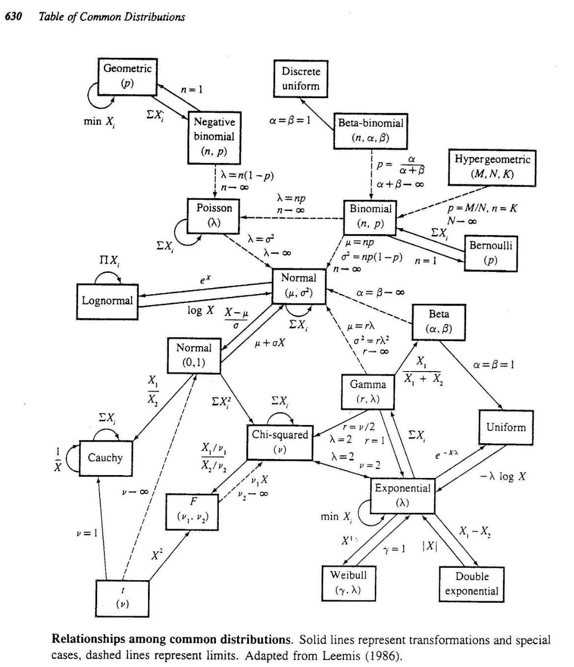
Lecturer-provided image, reproduced unchanged. The original caption reads “Relationships among common distributions” and credits an adaptation of Leemis (1986). Use this as a visual recap before moving to sampling uncertainty. Trace the relationships already covered: Bernoulli to binomial through sums, binomial to Poisson for rare events, binomial or Poisson to normal under suitable approximation conditions, and normal to log-normal by exponentiation. Each connection requires its stated parameter conditions and any relevant independence assumptions. The diagram includes further families and parameter conventions beyond this session; focus discussion on the models taught here. The full-size link allows students to inspect the smaller labels.
A new question: how stable is our estimate?
Let \(X_1, X_2, \ldots, X_n\) be a random sample from a population. For review times, \(X_i\) is the duration of review \(i\) .
The sample mean combines the \(n\) observations:
\[\bar{X}=\frac{X_1+X_2+\cdots+X_n}{n}=\frac1n\sum_{i=1}^{n}X_i.\]
Mean \(\mu\)
Sample mean \(\bar X\)
Variance \(\sigma^2\)
Sample variance \(s^2\)
Proportion \(p\)
Sample proportion \(\hat p\)
Observed values \(x_1, x_2, \ldots, x_n\) give a numerical estimate , such as \(\bar{x}\) .
Follow the original SOA-week5 notation: introduce the random observations X1, X2, …, Xn before writing their mean. Each Xi represents one observation; n is the sample size. The capital-letter mean is a random variable because its inputs are random. Once the observations take values x1, x2, …, xn, calculate the realised mean xbar=(x1+x2+…+xn)/n. For the examples and standard-error results below, the draws are independent from the same population. A parameter belongs to the population or process; an estimator is a rule applied to random data. Estimator bias, precision and consistency are developed further in Session 5 with confidence intervals. Do not define a point estimate as necessarily the most likely parameter value.
From a stable target to sampling uncertainty
Recall Session 3: with independent trials and constant \(p\) , the running proportion converges to \(p\) .
Law of large numbers Length of a growing sequence
Where does the running estimate settle?
Sampling distribution Which sample of a fixed size we observe
How much do estimates vary across samples?
A stable target can still produce different estimates in repeated samples.
Allow a brief retrieval before constructing a sampling distribution. Session 3 now introduces the LLN with the running-default-rate plot and the independence activity. Here, move from one growing sequence to repeated samples at a fixed n. The next slide uses sample means; the same distinction applies to proportions. Larger n concentrates an estimate nearer its target under the assumptions, while a sampling distribution quantifies its variation at each n.
Repeated samples give different means
Imagine a population with review times 4, 8, 12 and 16 minutes , each equally likely.
Draw \(X_1\) and \(X_2\) independently with replacement\(\bar{X}=(X_1+X_2)/2\) .
\(4,4\) \((4+4)/2=4\)
\(4,12\) \((4+12)/2=8\)
\(8,16\) \((8+16)/2=12\)
\(16,16\) \((16+16)/2=16\)
Repeat this process: the distribution of \(\bar X\) is its sampling distribution .
This small illustrative population makes the repeated-sampling mechanism visible before showing a CLT simulation. The four rows are selected examples, not a representative sample of all possible pairs. There are 4×4=16 equally likely ordered pairs. Sampling with replacement makes the draws independent and permits pairs such as (4,4). Each pair produces one mean; many pairs can produce the same mean.
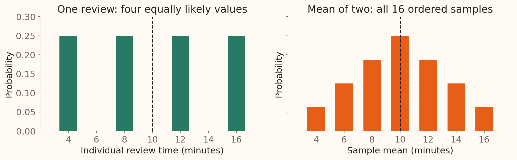
Individual values and means have different distributions
Both distributions have mean 10 minutes . The sample means cluster more tightly.
For example, four ordered pairs give \(\bar X=10\) , so \(P(\bar X=10)=4/16\) .
Enumerate (4,16), (8,12), (12,8) and (16,4). The population variance is 20 minutes squared, so SD(X)=sqrt(20)≈4.47 minutes. The variance of the two-observation mean is 10, so SD(Xbar)=sqrt(10)≈3.16 minutes. The sampling distribution is discrete and triangular here. It is not yet normal, and the SE formula does not require normality. The exact enumeration is stored in the numerical audit.
Standard error is the SD of an estimator
Let \(X_1, X_2, \ldots, X_n\) be independent observations from the same population, with \(E(X_i)=\mu\) and \(\operatorname{Var}(X_i)=\sigma^2<\infty\) .
For their sample mean \(\bar{X}=(X_1+X_2+\cdots+X_n)/n\) :
\[E(\bar X)=\mu,\qquad \operatorname{Var}(\bar X)=\frac{\sigma^2}{n},
\qquad SE(\bar X)=\frac{\sigma}{\sqrt n}.\]
For the two-review example:
\[SE(\bar X)=\frac{\sqrt{20}}{\sqrt2}=\sqrt{10}\approx3.16\text{ minutes}.\]
The mean estimates the same target; averaging reduces its variability.
Use Session 3’s sum and scaling rules: E(sum Xi/n)=nmu/n=mu, and Var(sum Xi/n)=n sigma²/n² because the independent variances add. These moment results hold without normal data. If sigma is unknown, estimate the standard error with s/sqrt(n); the distinction between known and estimated SE leads to the t procedure in Session 5. SE measures sampling spread, not a guarantee that one realised estimate lies within that distance of mu.
SD and SE answer different questions
Describes variation in…
Individual observations
Sample means
For review times
How different are individual times?
How different are repeated sample averages?
Increase \(n\) for the same population
Population SD stays the same
SE decreases
To halve SE , multiply the sample size by four .
Students often expect twice the data to halve uncertainty. Calculate SE(4n)=sigma/sqrt(4n)=SE(n)/2. Multiplying n by 9 divides SE by 3; multiplying it by 100 divides SE by 10. The population distribution remains fixed; the observed sample SD can fluctuate. Improving precision does not by itself fix selection bias or dependence.
Sampling a large share of a finite population
For a simple random sample without replacement , from \(N\) records:
Small fraction, such as \(n/N\le0.05\)
Correction is close to 1
Large fraction of the population
Less uncertainty about that population mean
All \(N\) records
No sampling uncertainty about that finite mean
The source calls this the finite population correction. Here sigma² is the finite-population variance defined with denominator N, with N>1. It adjusts for dependence induced by sampling without replacement. For the Session 2 bank example, N=800 and n=30 gives a correction sqrt(770/799)≈0.9817. An independently sampled process or sampling with replacement uses the preceding formula without this correction. Measuring every record removes sampling error for the finite-frame mean; measurement and coverage errors are separate issues. The 5% fraction is a practical approximation rule.
Larger samples make the mean more stable
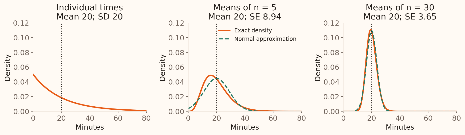
Each panel uses minutes on the same horizontal scale .
The individual distribution stays skewed; averages become tighter and more symmetric.
Illustrative exponential review-time model: mean = SD = 20 minutes. Orange: exact densities; green: normal approximations for sample means.
This is an exact mathematical illustration, not observed review data. The exponential distribution provides a simple positive, right-skewed population; students need not learn its formula here. Independent means have gamma densities with shape n and scale 20/n, plotted exactly. SE is 20/sqrt(n): 8.94 minutes at n=5 and 3.65 at n=30. The source’s individual spending versus average spending example motivates this comparison. The same axes show concentration; the next theorem explains standardised shape. Normal approximations can allocate some mass below zero, especially at small n.
Central limit theorem
Let \(X_1, X_2, \ldots, X_n\) be independent observations from the same distribution , with \(E(X_i)=\mu\) and \(0<\operatorname{Var}(X_i)=\sigma^2<\infty\) .
First form the sample mean :
\[\bar{X}=\frac{X_1+X_2+\cdots+X_n}{n}=\frac1n\sum_{i=1}^{n}X_i.\]
As \(n\to\infty\) , standardise the sum or, equivalently, the mean:
\[Z_n=\frac{(X_1+X_2+\cdots+X_n)-n\mu}{\sigma\sqrt n}
=\frac{\bar{X}-\mu}{\sigma/\sqrt n}\ \xrightarrow{d}\ N(0,1).\]
For sufficiently large \(n\) : \(\displaystyle \bar{X}\ \text{approximately follows}\ N\!\left(\mu,\frac{\sigma^2}{n}\right)\) .
Restore the original SOA-week5 sequence explicitly: individual observations X1, X2, …, Xn; their mean; then the equivalent standardised sum and mean. Independent observations from the same distribution are called independent and identically distributed (i.i.d.). Each observation has mean mu and finite positive variance sigma². Their sum has mean nmu and SD sigma sqrt(n), while their mean has mean mu and SE sigma/sqrt(n). Dividing the numerator and denominator of the standardised-sum expression by n gives the standardised-mean expression. Read the numerator as estimation error and the denominator as its standard error. The arrow denotes convergence in distribution: for each real z, P(Z_n<=z) tends to Phi(z). The unstandardised sample mean concentrates at mu as n grows; it does not converge to a normal distribution with a fixed positive variance. This corrects the misleading simplified limit in the source. Independent, identically distributed sampling and finite positive variance are sufficient conditions for the displayed classical CLT. The expectation and SE formulas already held before introducing this approximation.
Sampling distribution of \(\bar{X}\)
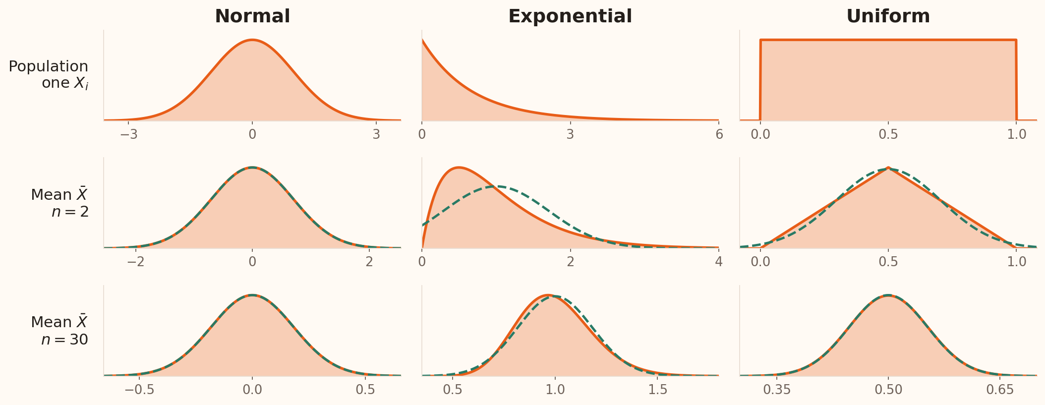
Read down each column: keep the population fixed and increase the sample size.
Different population shapes can give approximately normal sample means .
Restore the purpose of the original SOA-week5.tex slide “Sampling Distribution of Xbar” using its CLT-12-normal.png comparison of normal, exponential and uniform populations. This landscape version uses exact densities and retains n=2 and n=30 so all panels remain readable. For each column, repeatedly draw independent X1, X2, …, Xn from that one population and calculate Xbar=(X1+…+Xn)/n. Each lower curve is the distribution of the repeated means, not a changed population distribution. The normal population is N(0,1), so its mean is exactly N(0,1/n) at every n. Exponential observations have mean and SD 1; their average has a gamma density with shape n and scale 1/n, and skewness 2/sqrt(n), so n=30 is closer to normal but still not exactly normal. Uniform observations on [0,1] have mean 0.5 and variance 1/12; the average of two is triangular and the average of thirty is close to normal. Their exact mean density is n times the Irwin-Hall(n) density evaluated at n times the mean. Every matched normal curve has the same mean and variance as the corresponding sample mean. Horizontal and vertical scales change between panels to reveal shape; the previous common-axis review-time figure demonstrates shrinking spread. Ask students which column is exactly normal for n=2 and which is most skewed. Only the normal column is exactly normal; symmetry alone does not make the uniform n=2 mean normal. These are illustrative distributions, not observed bank data.
When is the normal approximation useful?
For independent \(X_1, X_2, \ldots, X_n\) from the same population:
Normal Exactly normal for every \(n\) , including small samples
Non-normal , with finite varianceApproximately normal for sufficiently large \(n\) ; \(n\ge30\) is a starting guide
Strong skew or outliers May need \(n\ge50\) or far more; inspect the approximation
Use the population mean and the variance of the mean :
\[\bar{X}\ \text{is exactly or approximately}\ \mathcal{N}\!\left(\mu,\frac{\sigma^2}{n}\right).\]
30 and 50 are guides. Check the fit for the probability you need.
This extends the original SOA-week5.tex “Distribution of Sample Mean” slide and connects each rule to the preceding population-shape comparison. For independent normal observations, the result is exact even for n=1 or n=2. For independent, identically distributed non-normal observations with finite positive variance, the CLT supports a normal approximation for sufficiently large n. The source’s 30 and 50 are planning heuristics, not universal thresholds or sharp boundaries; mild bounded distributions may be well approximated with fewer observations, while strong skew and rare extreme values may require far more. A uniform mean with n=2 is triangular despite being symmetric. In the exponential example, skewness of the mean is 2/sqrt(n), about 0.365 at n=30 and 0.283 at n=50, so convergence is gradual. Assess accuracy for the requested interval or tail, using an exact distribution when available or a suitable simulation; the next real-bank-balance figure illustrates this check. Finite positive variance and independence remain important: increasing sample size alone does not establish either assumption, and a larger biased sample can precisely estimate the wrong target. Dependence can change the variance of the mean and the conditions for a CLT. Calligraphic N denotes a normal distribution here, whereas capital N in the earlier finite-population formula denotes population size. Week 5 uses this distinction when selecting intervals for means.
Real bank balances: inspect the approximation
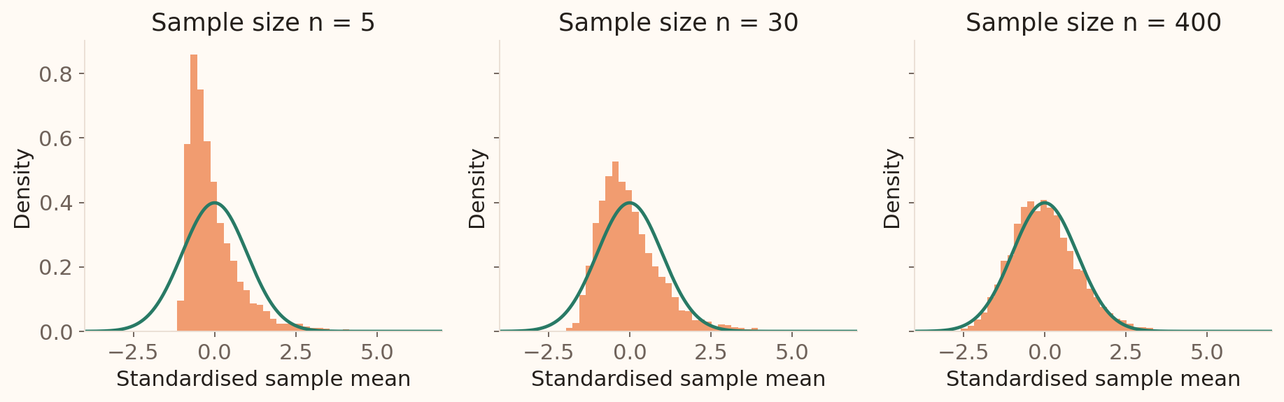
The CLT describes sample means . Individual balances keep their original skew.
6,000 samples with replacement at each size from UCI Bank Marketing , seed 202604. Green curve: standard normal density.
The plotted quantity is (sample mean − frame mean)/(frame SD/sqrt(n)). Strong skew can persist at moderate sample sizes; there is no universal sample-size cutoff that guarantees a good normal approximation. The resampling experiment here uses replacement, matching the independent draws assumed in the displayed SE formula.
One day’s error or a 25-day average?
Return to daily settlement errors: \(X_i\sim N(0,5^2)\) in £ thousands.
Assume 25 independent days from the same model .
Which is more likely: one day’s error exceeds £2,000 , or the 25-day average error exceeds £2,000?
Before calculating, identify the relevant spread:
Individual error: \(SD(X_i)=5\) .
Average error: \(SE(\bar X)=5/\sqrt{25}=1\) .
Allow a short prediction before the answer slide. Independence of daily errors is an assumption to check, not a property of the calendar. The question is about the average signed error; it is different from the total error, the average absolute error or at least one daily exceedance. Both distributions are exactly normal under this illustrative model.
Same threshold, different uncertainty
One error \(X_i\)
\(N(0,5^2)\) \(2/5=0.4\)
Average \(\bar X\) of 25 errors
\(N(0,1^2)\) \(2/1=2\)
\[P(X_i>2)=1-\Phi(0.4)=0.3446.\] \[P(\bar X>2)=1-\Phi(2)=0.0228.\]
Identify the random quantity first: its SD or SE determines the calculation.
The same £2,000 threshold is only 0.4 individual SDs above the mean, but two standard errors above the expected 25-day average. Point out that no large-sample approximation is needed here, because independent normal observations give an exactly normal mean at every n.
Separate customer variation from sampling uncertainty
For planning, suppose account balances have SD £3,000 .
Standard error of the mean
?
?
Calculate both standard errors. Does a larger sample make individual balances less variable or less skewed?
Allow two minutes of paired calculation, then use the worked debrief and closing CLT activity. Under independent sampling, SE values are £300 and £150. The distribution of the sample mean becomes tighter; the distribution of individual balances is unchanged. The finite variance and independence conditions matter. These rounded parameters are illustrative.
Sampling exercise: interpret the answer
With population SD £3,000 and independent observations:
\(n=100\) \(3{,}000/\sqrt{100}=£300\) £3,000
\(n=400\) \(3{,}000/\sqrt{400}=£150\) £3,000
Four times as many observations halves the spread of repeated sample means.
The individual balance distribution keeps its original spread and shape.
Debrief the distinction before the CLT activity. These rounded parameters describe an illustrative planning population; they are not the UCI balances, which are measured in euros. Ask students to explain why the third column stays fixed. If sigma is estimated from the observed sample, its estimate can vary, but the underlying population SD remains the same in this comparison.
What becomes approximately normal?
We draw independent samples from the same skewed balance distribution with finite variance. As sample size grows, what does the central limit theorem describe?
Individual balances become symmetric
The sampling distribution of the mean becomes approximately normal
The largest balance becomes normal
The sample mean equals the population mean every time
Format: multiple choice, one answer; 60 seconds. Correct: option 2. Debrief: the sampling distribution changes with n; the distribution of individual balances does not. Ask what happens to SE if sample size is multiplied by four: it halves under the same model.
Session 4 takeaway
Match the model to the process and its assumptions.
Continuous probabilities are areas; standardise normal outcomes.
Standard error describes how estimates vary across samples.
The CLT concerns sample means, not the shape of the original data.
Next: express sampling uncertainty with confidence intervals and assess benchmark claims.