Statistics for Analytics

Session 5: Estimation, Confidence Intervals & Testing

Dr Zexun Chen

Zexun.Chen@ed.ac.uk

Today’s route

Report plausible parameter values, then ask how the data compare with a benchmark.

Flexible estimate: 150 minutes of teaching plus a 10-minute break. Timings include calculation, discussion and activity debriefs. Outcomes: compare estimators using bias, variance and consistency; construct and interpret mean and proportion intervals; plan precision; select an alternative before analysing data; carry out one-sample z and t calculations; connect a matching interval and test.

• 000–005: retrieve Week 4 and define today’s estimation question.
• 005–020: proportion example, estimator properties and a concrete comparison.
• 020–045: normal-area construction and savings-account practice.
• 045–055: coverage, confidence width and Wooclap.
• 055–065: break.
• 065–090: t statistic, degrees of freedom, table, review-time exercise and real balances.
• 090–110: proportion interval, precision planning and Wooclap.
• 110–140: definitions, possible errors, testing steps, approval-time calculations and interval/test connection.
• 140–155: proportion testing, p-value Wooclap and real-data analysis guide.
• 155–160: synthesis and questions.

Week 4 has already developed sampling distributions, SE and the CLT. Retrieve these on one slide, then distinguish parameter, estimator and estimate using a proportion example. Connect estimator properties to interval construction. Begin testing with the loan-approval question. Introduce hypothesis testing, possible errors and the two decision approaches, then return to the example for the worked solution. Session 6 applies these procedures to real data, paired differences, error costs and power.

Estimates & Uncertainty

Case: estimating mean customer balance

Question: How precisely can 400 records estimate a bank’s mean recorded balance?

Part of the problem	This classroom exercise
Population frame	45,211 historical campaign records
Random sample	400 records, selected without replacement
Point estimate	Sample mean balance: €1,517.92
Target	Mean balance across the full frame

UCI Bank Marketing, bank-full.csv, sample seed 11624. Treat the published records as the population for this exercise.

Two forms of inference

Estimation

What parameter values are plausible?

Hypothesis testing

Is a particular claim compatible with the data?

We will estimate a plausible range, then use the same sampling model to assess a benchmark.

Retrieve Week 4: parameter, estimator, estimate

Parameter	Estimator
Population mean \(\mu\)	Sample mean \(\bar X\)
Population variance \(\sigma^2\)	Sample variance \(s^2\)
Population proportion \(p\)	Sample proportion \(\hat p\)

A point estimate is the numerical value obtained from the observed sample.

For the balance case: target \(\mu\), rule \(\bar X\), observed estimate \(\bar x=€1{,}517.92\).

Retrieve rather than reteach: Week 4 distinguished random observations, a rule applied to them and its realised value. The mean has SE sigma/sqrt(n); estimating sigma gives s/sqrt(n). Today we use that uncertainty to construct intervals and tests. In this table s² denotes the usual sample variance with denominator n−1.

Loan defaults: parameter, estimator, estimate

A bank observes 20 defaults among 400 sampled loans over one year. What is our estimate of the population default rate?

Concept	Notation or value	Meaning
Parameter	\(p\)	Unknown population default rate
Estimator	\(\hat p=D/n\)	Default count \(D\) divided by sample size \(n\)
Estimate	\(20/400=0.05=5\%\)	Numerical value from the observed sample

The population rate \(p\) is fixed; another sample can give a different estimate \(\hat p\).

Illustrative loan sample; assume representative selection and a common one-year observation period.

Allow about two minutes within the opening estimation block. Ask students to identify the population target, calculation rule and observed result before reading the table. D is a random default count before observing the sample; here its realised value is 20 and n=400. The notation p-hat is conventionally used for both the estimator and its realised estimate, so the distinction comes from whether we mean the rule or the observed number.

The estimate 0.05 does not establish that the population parameter equals 0.05. In Week 4’s RBS binomial example, p=0.05 was an assumed model input; here 20/400 is an observed sample summary in a separate illustrative estimation exercise. Another sample with 16 defaults would give 16/400=0.04 while the population target remains the same. Define a consistent population and one-year horizon before comparing rates.

Connect to Bernoulli indicators: let I_i=1 for a default and 0 otherwise, so D=sum I_i and p-hat=(I_1+…+I_n)/n is the sample mean of binary observations. Under independent observations with common probability p, D follows Bin(n,p). This connection prepares the later proportion interval; the present slide focuses on parameter, estimator and estimate. This extends the preceding parameter–estimator recap to a proportion. Later in this session, sampling uncertainty in a proportion leads to a confidence interval.

Bias and precision

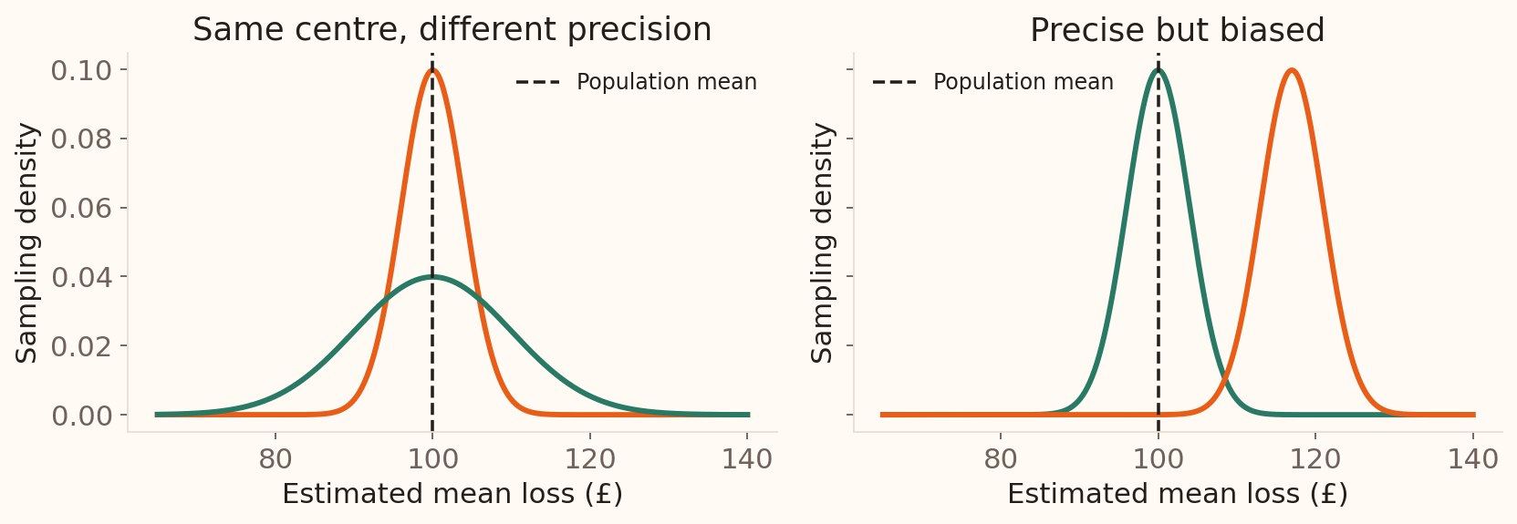
Bias shifts the centre away from the target; precision describes how tightly estimates cluster.

Illustrative estimator distributions; the dashed line marks a hypothetical true mean loss of £100.

What makes an estimator useful?

Property	Mathematical statement	Meaning
Unbiasedness	\(E(\hat\theta)=\theta\)	Correct centre across repeated samples
Precision	Small \(\operatorname{Var}(\hat\theta)\)	Estimates cluster closely
Consistency	\(\hat\theta_n\xrightarrow{P}\theta\)	Concentrates near the target as \(n\) grows

Compare efficiency among estimators of the same parameter, under the same model.

Read convergence in probability as: for every fixed positive tolerance, the chance of an estimation error larger than that tolerance tends to zero. Relative efficiency usually compares variance within an unbiased class; specify the model and class before calling an estimator efficient. A narrow sampling distribution can be centred on the wrong value. The next example separates these properties without new distribution theory.

Compare three rules for estimating a mean

Take independent observations with common mean \(\mu\) and variance \(\sigma^2\).

Estimator	Expected value	Variance
First observation \(X_1\)	\(\mu\)	\(\sigma^2\)
Sample mean \(\bar X\)	\(\mu\)	\(\sigma^2/n\)
Shifted mean \(\bar X+£10\)	\(\mu+£10\)	\(\sigma^2/n\)

At \(n=25\): \(\operatorname{Var}(\bar X)=\sigma^2/25\), so \(SD(\bar X)=\sigma/5\).

Discuss: as \(n\) grows, which rule concentrates around \(\mu\)? Which stays too high? Which ignores the extra observations?

Allow about four minutes across this comparison and the next slide: predict, then read the visual debrief. Assume observations are balances in pounds from an illustrative population with finite positive variance. X1 and the sample mean are unbiased, but only the sample mean becomes consistent as n increases. X1 ignores the additional observations. The shifted mean becomes concentrated around mu+10, so its bias remains £10 and it is inconsistent for mu. Both means have the same variance: precision alone cannot identify the right target. These conclusions reuse Week 3’s expectation/variance rules and the Week 4 law-of-large-numbers retrieval. Increasing sample size addresses sampling spread, while improved collection is needed for selection bias.

More data: which estimate approaches the target?

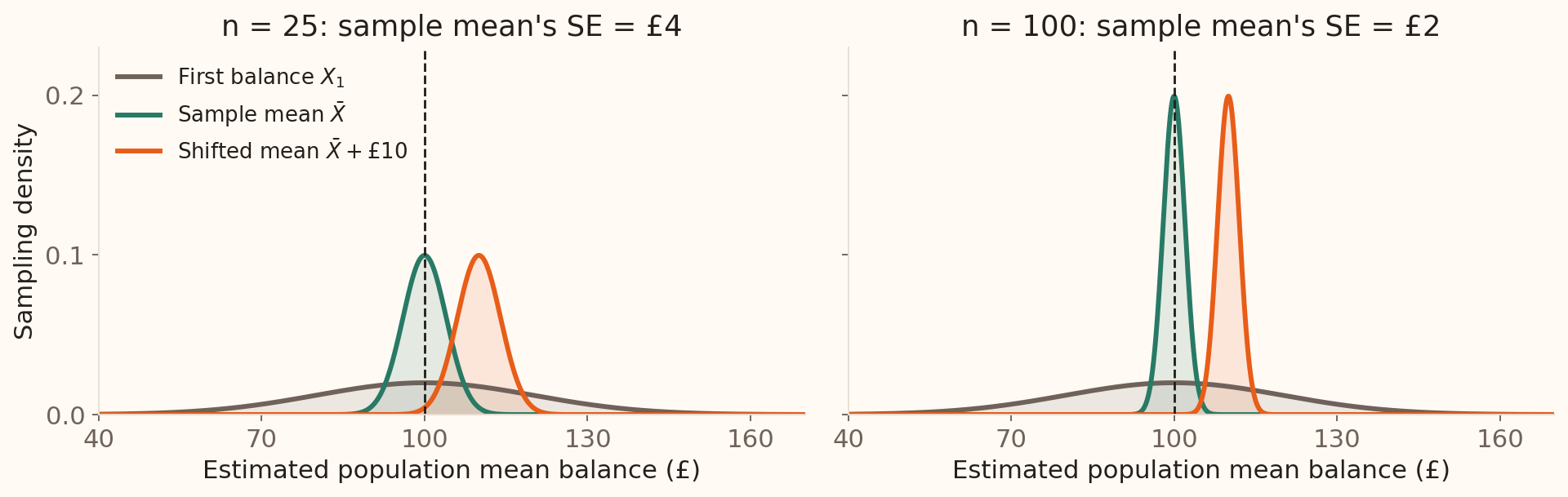
• \(X_1\): stays equally variable; it ignores the extra observations.
• \(\bar X\): concentrates around £100, the true mean.
• \(\bar X+£10\): concentrates around £110; its bias stays £10.

Illustrative independent normal balances: mean £100, SD £20. Curves are exact sampling densities; dashed line = true mean. Both panels use the same scales.

Debrief the discussion on the comparison slide. Grey is the first-observation estimator, green the sample mean, and orange the shifted mean. The grey curve is unchanged because increasing n does not change the first observation’s distribution. For n=25, both averages have variance 16 and SD 4; for n=100, their variance is 4 and SD 2. The green curve concentrates on the target £100. The orange curve becomes equally precise but remains centred £10 above the target. Thus the sample mean is consistent; the shifted mean is inconsistent for mu, and the first-observation estimator is unbiased but inconsistent. The taller peaks reflect narrower probability distributions, not more probability in total: each curve integrates to one. The curves show distributions of estimates across repeated samples, not a histogram of the 25 or 100 individual balances. Negative balances are permitted in this illustrative normal account-balance model. A shifted estimate can become closer to the target on average as its variance shrinks, but its fixed bias persists.

Confidence Intervals

How far could our estimate be from the target?

Week 4 gave the sampling distribution of the mean:

\[\bar X\approx N\!\left(\mu,\frac{\sigma^2}{n}\right).\]

If this model is appropriate, approximately 95% of sample means lie within 1.96 standard errors of \(\mu\).

We observe \(\bar x\), but \(\mu\) is unknown. Can we turn this probability statement into an interval for \(\mu\)?

Connect the inference question to Week 4’s normal-area and sampling-mean calculations. Under independent normal observations this distribution is exact. Otherwise it is a large-sample approximation under the CLT conditions. The following construction assumes known sigma; uncertainty from estimating it is developed after the break. This is a statement about the mean across samples, not the spread of individual balances.

Where does 1.96 come from?

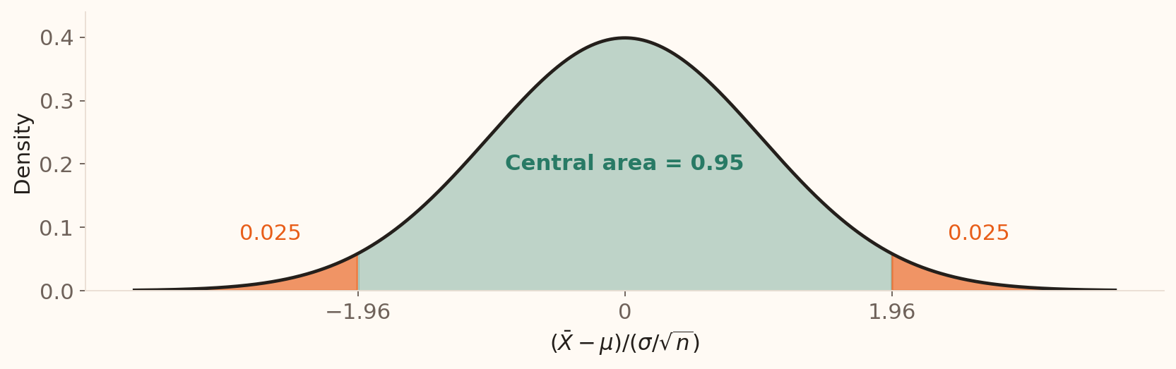
\[P\!\left(-1.96\le\frac{\bar X-\mu}{\sigma/\sqrt n}\le1.96\right)\approx0.95.\]

Split the remaining 5% equally between the two tails.

Retrieve Phi(1.96)=0.975 and Phi(−1.96)=0.025 from Week 4’s normal table. The 95% central area is 0.975−0.025. For general confidence 1−alpha, the upper critical value is Phi inverse of 1−alpha/2. Distinguish a tail area from the corresponding z value. All figures here show mathematical models, not empirical bank data.

Rearrange the event to enclose the unknown mean

1. Start with the standardised distance: \[-z^*\le\frac{\bar X-\mu}{\sigma/\sqrt n}\le z^*.\]

2. Multiply by the standard error: \[-z^*\frac{\sigma}{\sqrt n}\le\bar X-\mu\le z^*\frac{\sigma}{\sqrt n}.\]

3. Rearrange to put \(\mu\) in the middle: \[\boxed{\bar X-z^*\frac{\sigma}{\sqrt n}\le\mu\le\bar X+z^*\frac{\sigma}{\sqrt n}}.\]

The endpoints vary across samples; the parameter stays fixed.

Write each inequality separately if needed: xbar−mu≤zSE gives mu≥xbar−zSE, and xbar−mu≥−zSE gives mu≤xbar+zSE. The confidence statement follows because this is the same event as the preceding central-area statement. Before sampling the endpoints are random; after sampling they are two observed numbers.

The interval template

\[\text{estimate}\ \pm\ \text{critical value}\times SE\]

Component	Role
Estimate	Centre
Standard error	Sampling uncertainty
Critical value	Desired confidence

Mean with known \(\sigma\)

When population standard deviation is known:

\[\bar X\pm z^*\frac{\sigma}{\sqrt n}\]

Confidence	\(z^*\)
90%	1.645
95%	1.960
99%	2.576

Savings accounts: calculate an interval

A bank takes a random sample of 100 savings accounts.

\[\bar x=£1{,}500,\qquad \sigma=£300.\]

Assume independent observations and an adequate normal approximation for the sample mean.

1. Calculate the standard error.
2. Find the 95% margin of error.
3. Write the interval and identify its population target.

Illustrative savings-account scenario. The population SD is assumed known for this exercise.

Allow three minutes of individual or paired calculation before showing the answer. Treat the sampling fraction as negligible. The target is the population mean savings-account balance, not the balance of a particular customer. Use pounds throughout. Historical information can supply a planning SD, but an estimated historical value is not automatically a known population SD.

Savings accounts: work through the answer

1. Standard error: \[SE=\frac{300}{\sqrt{100}}=£30.\]

2. Margin of error: \[ME=1.96\times30=£58.80.\]

3. Confidence interval: \[1500\pm58.80=\boxed{(£1{,}441.20,\ £1{,}558.80)}.\]

The estimated population mean balance is £1,500, with a 95% confidence interval from £1,441.20 to £1,558.80.

Critical value 1.96 is rounded from the normal quantile; both endpoints round to the displayed values. Compare SE £30, margin £58.80 and individual balance SD £300. Ask why the interval uses the smaller quantity: it estimates a mean. Interpret the confidence level using repeated sampling on the next slides.

Confidence is long-run coverage

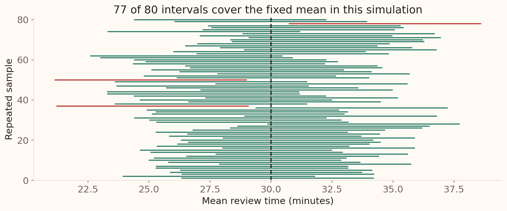
Over many repetitions, a 95% procedure covers the fixed parameter about 95% of the time.

Simulation: normal review times, mean 30 minutes, known SD 12, samples of 36, seed 202605. Finite runs need not give exactly 95% coverage.

The interval is random before sampling; the population parameter is fixed. A realised frequentist interval either contains that parameter or does not. It is not an interval containing 95% of individual review times, nor does nominal coverage account for biased collection or an invalid model.

Higher confidence gives a wider interval

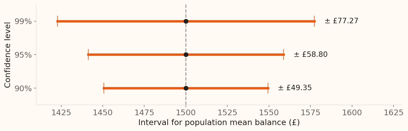
The sample and standard error stay the same. A larger critical value gives greater coverage and less precision.

The plot uses unrounded normal critical values. Keep the centre £1,500 and SE £30 fixed. The 99% interval has greater long-run coverage, but includes a wider range of possible mean balances. To increase confidence while keeping the margin fixed, collect more observations; sample-size planning follows later.

Interpret 95% confidence

Which statement correctly describes a 95% confidence-interval procedure under its assumptions?

1. 95% of individual account balances fall in the interval
2. About 95% of intervals from repeated samples contain the fixed population mean
3. The sample mean has a 95% chance of being correct
4. The interval removes selection bias

Format: multiple choice, one answer; 90 seconds. Correct: option 2. Debrief with the coverage plot: intervals vary while the parameter stays fixed; a finite simulation need not cover exactly 95% of the time.

Estimating the SD

When \(\sigma\) is unknown

Replace \(\sigma\) with sample SD \(s\) and use Student’s t distribution:

\[\bar X\pm t^*_{n-1}\frac{s}{\sqrt n}\]

The t distribution accounts for estimating \(\sigma\).

Why does estimating the SD change the distribution?

With independent normal observations:

\[Z=\frac{\bar X-\mu}{\sigma/\sqrt n}\sim N(0,1),\qquad T=\frac{\bar X-\mu}{S/\sqrt n}\sim t_{n-1}.\]

The estimated denominator changes from sample to sample, adding uncertainty.

Student’s t distribution allows for estimating the population SD from the same sample.

Capital S emphasises that the sample SD is random; lowercase s is its observed value. A small denominator can produce a large absolute t statistic, contributing to heavier tails. Under independent normal sampling, (n−1)S²/sigma² is chi-square with n−1 df and independent of the sample mean; this gives the exact t result. For non-normal observations the usual t interval relies on a suitable approximation; t does not itself remove skewness or dependence.

Why \(n-1\) degrees of freedom?

The deviations from the sample mean satisfy

\[\sum_{i=1}^{n}(x_i-\bar x)=0.\]

If three deviations are −2, +1, and ?, the last must be +1.

Once the mean is fitted, only \(n-1\) deviations can vary freely.

Connect this to Week 2’s sample variance denominator. Knowing any n−1 deviations determines the remaining one because their sum is zero. This supplies the degrees of freedom for estimating a single population variance around an estimated mean. It is a degrees-of-freedom explanation, not a full proof of the t distribution.

Normal versus t

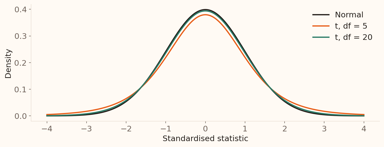
As \(df\) increases, \(t^*\) approaches the corresponding normal critical value.

Find a t critical value: row, column, cutoff

Each entry is a cutoff \(t^*\); the column heading gives the upper-tail probability \(P(T>t^*)\).

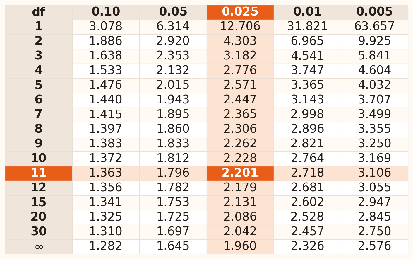
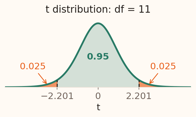
95% interval, \(n=12\):

1. Row: \(df=12-1=11\).
2. Column: \(0.05/2=0.025\).
3. Read: \(t^*=\mathbf{2.201}\).

Selected rows; values rounded to three decimals. A cumulative table labels the same column 0.975; a two-sided confidence table labels it 95%.

Allow about two minutes. The normal cumulative table takes z and returns a probability; this t table takes degrees of freedom and an upper-tail probability and returns a cutoff. For a 95% two-sided interval, 1−0.95=0.05 lies outside the central area, with 0.025 in each tail. Trace row 11 across to column 0.025 and read 2.201. By symmetry the lower cutoff is −2.201. Row 12 would use the sample size rather than its degrees of freedom. Column 0.05 gives 1.796 and leaves 0.05 in each tail, giving only 90% central coverage. Ask students to find the cutoff for n=12 and 99% confidence: row 11, upper tail 0.005, t*=3.106. A one-sided upper test at 5% instead uses column 0.05. The infinity row gives the normal limit. The displayed cutoffs are rounded. Continue directly to the review-time interval using the same sample size and confidence level.

A small sample of review times

An analyst randomly selects 12 independent loan reviews from a stable process.

\[\bar x=8\text{ minutes},\qquad s=4\text{ minutes}.\]

Assume the population of review times is approximately normal.

1. Choose the reference distribution and degrees of freedom.
2. Calculate a 95% interval for the mean review time.
3. Explain why a small sample makes the shape assumption important.

Illustrative loan-review scenario.

Allow three minutes before the answer. The normal model is an approximation for this positive duration. In an actual process, examine the data for strong skewness and extreme observations before relying on a small-sample t interval. The summaries are supplied for this calculation exercise.

Review times: calculate and interpret

1. Use Student’s t with \(df=12-1=11\): \(t^*=2.201\).

2. Calculate the standard error and margin: \[SE=\frac4{\sqrt{12}}=1.155,\qquad ME=2.201(1.155)=2.542.\]

3. Construct the interval: \[8\pm2.542=\boxed{(5.46,\ 10.54)\text{ minutes}}.\]

The interval estimates the population mean. Individual reviews can lie outside it.

Calculate using unrounded SE and critical value, then round endpoints. The margin is approximately 2.5415. A normal critical value would produce the narrower interval 5.74–10.26; the larger t multiplier accounts for estimating sigma. These statements describe the procedure under the stated model.

Real campaign balances: \(\sigma\) unknown

Return to the opening 400-record sample: \(\bar x=€1{,}517.92\). Use the sample SD \(s=€2{,}842.26\) and \(df=399\):

\[SE=2842.26/\sqrt{400}=142.11\]

\[95\%\ CI=1517.92\pm1.966(142.11)\]

\[=(1238.53,1797.30).\]

Source: UCI Bank Marketing; reproducible 400-record sample, seed 11624. Strong balance skew makes the large sample important.

Choose normal or t: a practical guide

For a population mean, first ask whether the population SD is known.

Information	Which critical value?
Population SD \(\sigma\) known	Use normal (\(z\)).
SD estimated by \(s\), with \(n<30\)	Use \(t\), with \(df=n-1\).
SD estimated by \(s\), with \(n\ge30\)	\(t\) remains the standard choice; normal is a rough shortcut as \(n\) grows.

For 95% confidence, a quick large-sample calculation is estimate \(\pm\,2\times SE\).

Our examples: 12 reviews → \(t^*=2.201\); 400 balances → \(t^*=1.966\approx1.96\).

The t distribution approaches normal for larger degrees of freedom. The n=30 division is a teaching guideline, not a mathematical boundary. At n=30, df=29 gives a 95% t critical value about 2.045, compared with normal 1.960; the difference shrinks as n grows. When sigma is estimated, t remains the general method used in the worked examples; a normal multiplier is an explicitly approximate shortcut. For a known sigma use SE=sigma/sqrt(n), and for an estimated sigma use SE=s/sqrt(n). A historical SD estimate is still an estimate. The next slide explains when the population shape makes the approximation reasonable. These choices concern means; the proportion interval later uses its success/failure count check.

For sampling without replacement from a substantial share of a finite frame, recall Week 4’s finite population correction. For the 400 of 45,211 balance example its multiplier is 0.9956, so the displayed large-frame approximation changes little. The historical data support a finite-frame exercise; other populations require a justified sampling or process model.

How large should the sample be? A rough guide

For a mean, assume random sampling and independent observations. Then check the population’s shape.

Sample size	Practical guide
Below 15	Use a small sample when the population is approximately normal, with no strong outliers.
15–29	Rough symmetry and no strong outliers can make the mean interval reasonable.
30 or more	A normal approximation for the mean is often reasonable with moderate skewness.
Strong skew or outliers	50 or more is a starting point; more data may be needed.

12 reviews: the normality assumption matters. 400 balances: averaging helps with skewness.

Required sample size depends on the population; 30 or 50 observations do not guarantee accuracy.

Allow about two minutes. Use the 15, 30 and 50 guidelines as a practical first check. The strong-skew row takes priority over the ordinary n>=30 guideline. A normal approximation here describes the sampling distribution of the mean; increasing n does not make the individual observations normal. The CLT assumes suitable sampling conditions and finite variance, and convergence can be slow for strongly skewed or heavy-tailed populations. The t interval is exact under independent normal sampling. For small non-normal samples, rough symmetry without strong outliers can make it a useful approximation.

The loan-review exercise assumes random, independent observations from an approximately normal population; its summaries alone cannot verify those assumptions. Plot the times and examine the collection process. In the 400-record balance sample, check whether a few extreme balances dominate the mean and SD. The small sampling fraction makes the finite-frame correction negligible for the displayed precision.

Optional discussion: would 400 reviews from only the fastest team give a reliable interval for the whole bank? No: more observations can narrow the interval while leaving selection bias. Reviews for the same customer or under shared working conditions may also be positively correlated, so s/sqrt(n) can understate uncertainty. Sample across the target process and account for clustering. Sample-size guidelines address distributional approximation, while random selection and independence address how the observations were obtained.

Proportions & Precision

Interval for a proportion

A proportion is the fraction with a particular outcome: 800 satisfied customers out of 1,000 = 0.80 = 80%.

We use the sample proportion \(\hat p\) to estimate the population proportion \(p\).

\[\hat p\pm z^*\sqrt{\frac{\hat p(1-\hat p)}{n}}\]

For this normal approximation, check independence and at least 10 in each group: satisfied and not satisfied.

Retrieve the earlier loan-default example: the proportion is a count divided by the total, with values between zero and one. Multiply by 100 to express it as a percentage. Here p is the unknown fraction of all customers who are satisfied; p-hat is the observed fraction in the sample. A single response is yes/no, while the interval describes the population rate. This is the introductory Wald interval. Check for at least 10 successes and 10 failures before using the normal approximation. Total n alone is insufficient: for example, 2 satisfied responses out of 100 fail the check. For small counts or proportions near zero or one, use a method such as the Wilson interval rather than relying on this approximation.

Customer satisfaction: estimate the rate

A random survey of 1,000 customers finds 800 satisfied.

\[\hat p=800/1000=0.80.\]

There are 800 successes and 200 failures, so both observed-count checks exceed 10.

Calculate: the standard error, then a 95% confidence interval for the population satisfaction rate.

Illustrative customer survey. Assume independent, representative responses and a small sampling fraction.

Allow two minutes of calculation. The target is the rate among the bank’s defined customer population during the survey period. A Bernoulli outcome has variance p(1−p); Week 4 gives the variance of its sample proportion as p(1−p)/n. For this interval, replace the unknown p with the observed proportion. Nonresponse and coverage still need design attention.

Customer satisfaction: work through the interval

1. Estimate the standard error: \[\widehat{SE}=\sqrt{\frac{0.80(0.20)}{1000}}=0.01265.\]

2. Find the margin and interval: \[ME=1.96(0.01265)=0.02479,\] \[0.80\pm0.02479=\boxed{(0.7752,\ 0.8248)}.\]

The estimated satisfaction rate is 80%, with an approximate 95% interval of 77.52% to 82.48%.

Interpret: the margin is 2.48 percentage points. Does this interval describe individual responses?

An individual’s satisfaction outcome is binary; the interval estimates a population rate. Use 2.48 percentage points for the absolute margin, rather than a 2.48% relative error. The Wald interval works here as a large-sample approximation with a rate away from zero and one. Ask students to identify one design problem a narrow interval cannot repair.

Precision means a smaller margin of error

Our customer survey gave 80% satisfied, with a 95% interval from 77.52% to 82.48%.

Estimate \(\pm\) margin of error: 80% \(\pm\) 2.48 percentage points.

The margin tells us how far the interval extends on either side of the estimate.

More precision means a smaller margin, keeping the confidence level fixed.

Discuss: which survey result is more precise: 80% \(\pm\) 5 points or 80% \(\pm\) 2.5 points?

Answer: plus or minus 2.5 percentage points is more precise, because its interval is narrower at the same confidence level. The corresponding intervals are 75%–85% and 77.5%–82.5%. Precision concerns sampling uncertainty; an interval can be narrow even when selection is biased. The observed 80% estimate could change in a new survey. The following planning slide concerns choosing sample size before collecting those responses.

The general mean-planning formula is retained here for reference: ME=z* sigma/sqrt(n), so n>= (z* sigma/ME)^2. With sigma=£300, ME=£50 and z*=1.96, this gives n>=138.2976; round up to 139 records. A pilot SD can provide a planning value when the population SD is unknown. Confidence, variability and design determine the required sample size.

How many responses for a useful percentage?

Suppose we want to estimate the percentage of satisfied customers with 95% confidence.

Completed responses	Rough planning margin
100	\(\pm\) 10 percentage points
400	\(\pm\) 5 percentage points
1,600	\(\pm\) 2.5 percentage points

To halve the margin, collect four times as many responses.

Approximate 95% planning guide: independent random responses, a small sampling fraction, and a conservative planning rate of 50% satisfied.

Allow about two minutes. A proportion is a fraction or percentage with a yes/no outcome. Planning its precision means choosing how many responses to collect for a desired margin in percentage points. The 50% planning value is used when the satisfaction rate is unknown: p(1−p) is largest at p=0.5. It is a conservative input for planning, not a prediction that exactly half the customers will be satisfied.

For a quick calculation, round the 95% normal critical value 1.96 to 2. Combining that shortcut with p=0.5 gives m approximately 2 sqrt(0.25/n)=1/sqrt(n), in proportion units, or 100/sqrt(n) percentage points. Thus n=100, 400 and 1600 give planning margins of 10, 5 and 2.5 percentage points. The full planning expression is n>= (z)^2 p(1−p)/m^2. With z*=1.96 and m=0.05 it gives 384.16, rounded up to 385; the classroom shortcut rounds this to 400. At these three sample sizes, the unrounded-normal planning margins are about 9.80, 4.90 and 2.45 percentage points. These are approximate design calculations, not guaranteed coverage bounds for every population rate.

The sample size counts completed responses. Invitations may need to exceed that number because of nonresponse, and response bias still needs attention. The preceding 80%-satisfied example uses its observed proportion to estimate uncertainty after sampling; its margin can be smaller than this conservative planning guide. Keep confidence, planning rate and sampling design fixed for the fourfold rule. This table is a simplified derivation from the normal margin, while the earlier 15/30/50 sample-size guidelines apply to means. Neither replaces the success/failure count check when calculating a proportion interval.

Precision is a design choice

Change	Interval effect
Higher confidence	Wider
Larger sample	Narrower
More variability	Wider
Biased collection	Not repaired

Statistical precision and data quality are different dimensions.

Plan a more precise survey

A survey uses 100 responses. Keeping confidence and the planning variability fixed, how many responses are needed to halve the margin of error?

1. 150
2. 200
3. 400
4. 800

Format: multiple choice, one answer; 60 seconds. Correct: option 3. Debrief: margin is proportional to 1/sqrt(n), so halving it requires four times as many responses. Discuss why increasing n still does not repair a biased response process.

Testing a Mean

Loan approvals: has the mean time changed?

A bank’s benchmark mean approval time is 5 days. After a process change, a random sample gives

\[n=36,\qquad\bar x=4.7\text{ days}.\]

For the first calculation, assume known \(\sigma=1.5\) days and a suitable normal sampling model.

The observed mean is 0.3 days below the benchmark. Is that difference large relative to sampling uncertainty?

Illustrative loan-approval scenario. The 5-day benchmark is treated as fixed.

Ask students for an initial judgement: does a sample mean below 5 days establish that the population mean has changed? Use their answers to motivate a formal hypothesis test, then return to the calculation after introducing the two decision approaches. Define the parameter as the population mean approval time under the current process. Independent sampling and the assumed reference model are needed. The comparison addresses a benchmark; a before/after narrative alone does not isolate the causal effect of the process change. If the benchmark were estimated from another sample, its uncertainty would need to be included.

Hypothesis testing

Hypothesis testing uses sample evidence to decide whether a statement about a population parameter should be rejected.

Term	Meaning
Null hypothesis, \(H_0\)	A statement about the parameter that we use as the reference for the test.
Alternative hypothesis, \(H_A\)	The competing statement for which we seek evidence; it can be one-sided or two-sided.
Significance level, \(\alpha\)	A limit chosen in advance on the probability of rejecting a true \(H_0\).

We use \(\alpha=0.05\) in the following examples.

Allow two minutes. A hypothesis concerns a population parameter, such as a mean approval time or a satisfaction proportion. It is not a statement about the observed sample mean, which is already known. The null and alternative specify the competing parameter values. The alternative is also commonly written H1. A test assesses whether the sample evidence is sufficiently incompatible with the null model to reject it at the chosen level. Statistical rejection is a decision under the model and sampling assumptions, rather than proof of a claim. The next slide explains why even a correctly calibrated procedure can make a mistake.

Everyone can make a mistake

Suppose we test whether mean loan-approval time has fallen below 5 days:

\[H_0:\mu\ge5,\qquad H_A:\mu<5.\]

Random sampling can lead to either of two mistakes.

Error	What happens in this example?
Type I: false alarm	We conclude that approvals are faster when the true mean is still 5 days or more.
Type II: missed improvement	We fail to detect a reduction when the true mean is below 5 days.

An unusual sample can occur under a true null; a real change can be obscured by sampling variation.

Allow two minutes. Ask students to state which hypothesis is true in each row before naming the decision. Rejecting H0 supports the planned decrease; failing to reject means the evidence does not establish that decrease. The first error can trigger adoption of an ineffective process; the second can delay adoption of a useful change. These are illustrative consequences, not causal conclusions established by this one-sample test. A Type II error means failing to reject a false null, rather than establishing or accepting the null as true. Session 6 develops the truth table, error probabilities, power and operational consequences.

Steps of hypothesis testing

1. State the claim: identify the population parameter, \(H_0\) and \(H_A\); choose one or two tails.
2. Plan the test: choose \(\alpha\), the sampling model and the test statistic; check the assumptions.
3. Collect and calculate: obtain the sample and calculate the statistic.
4. Make the comparison: use a critical value or a p-value.
5. Report the conclusion: reject or fail to reject \(H_0\), and explain the estimated effect in context.

Choose the question, direction and significance level before examining the result.

Allow two minutes. The same first three steps lead to either decision approach on the next slides. Critical values are determined by the planned direction, alpha and reference distribution. A p-value is calculated from the observed statistic under that same null reference. Both approaches give the same decision when these ingredients match. The report should include the estimate, uncertainty, assumptions and population to which the result applies. When analysing an existing dataset, specify the question and analysis before inspecting the outcome comparisons; label questions suggested by the data as exploratory.

Critical-value approach: the rejection region

A critical value marks the boundary of the rejection region under \(H_0\).

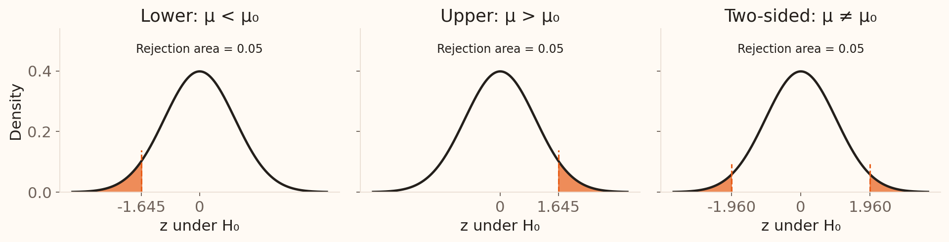
Reject \(H_0\) if the observed statistic falls in the shaded region.

At \(\alpha=0.05\), a two-sided test places 0.025 in each tail.

Allow three minutes. Choose the direction, significance level and reference distribution before using the observed statistic. For a normal test at alpha=0.05, reject below −1.645 for a lower-tail alternative, above 1.645 for an upper-tail alternative, or beyond ±1.960 for a two-sided alternative. Each picture has total rejection probability 0.05 under the boundary null. Ask which picture matches fallen, increased and changed.

For a t test, obtain the cutoffs from the t table with the relevant degrees of freedom. Compare a test statistic with a critical value on the same standardised scale; alpha is a probability, not a statistic cutoff. Shading here represents the rejection region fixed by alpha. The p-value shading later begins at the observed statistic. In a continuous model, including or excluding an exact cutoff does not change its probability. Values shown are rounded; use consistent precision near a boundary.

P-value approach

A p-value is the probability, under \(H_0\) and its assumptions, of a result at least as extreme as the observed result in the direction or directions specified by \(H_A\).

Compare the p-value with \(\alpha\)	Decision
\(p\le\alpha\)	Reject \(H_0\).
\(p>\alpha\)	Fail to reject \(H_0\).

Use this rule for both one-sided and two-sided tests. A two-sided p-value already includes both tails.

A small p-value indicates greater incompatibility between the data and the null model.

Allow three minutes. First use the statistic to calculate the appropriate null tail probability; then compare that probability with alpha. The p-value is conditional on H0 and the model assumptions. It is not the probability that H0 is true, the chance that the result is wrong, or the size of the effect. For a two-sided normal or t test, double the smaller one-tail probability; this construction uses the symmetry of these reference distributions. Compare the resulting full p-value with alpha. The alpha/2 split is used to find two-sided critical values, not to halve the threshold for a fully calculated two-sided p-value. Failing to reject leaves the null compatible with the evidence without proving it true.

State the hypotheses before analysing the data

Planned question	Null hypothesis	Alternative
Has mean time changed?	\(H_0:\mu=5\)	\(H_A:\mu\ne5\)
Has mean time fallen?	\(H_0:\mu\ge5\)	\(H_A:\mu<5\)
Has mean time increased?	\(H_0:\mu\le5\)	\(H_A:\mu>5\)

Hypotheses describe the population mean. For the one-sided tests, calculate at the boundary \(\mu_0=5\).

Choose the scientific direction before seeing the observed mean. We compare the planned questions using the same numbers to explain how their tail areas differ, not to choose whichever produces a smaller p-value. The boundary gives the largest rejection probability within these one-sided normal-model nulls. An observed sample mean is already known and is not the unknown hypothesis target.

Approval times: standardise the observed difference

1. Standard error under the benchmark model: \[SE_0=\frac{1.5}{\sqrt{36}}=0.25\text{ days}.\]

2. Test statistic: \[z=\frac{\bar x-\mu_0}{SE_0}=\frac{4.7-5}{0.25}=\boxed{-1.20}.\]

The observed mean is 1.2 standard errors below the benchmark.

For the planned decrease, \(-1.20>-1.645\): the statistic is outside the critical region, so fail to reject \(H_0\).

Retrieve standardisation from Week 4. Here the relevant spread is the standard error 0.25, not the observation SD 1.5. Under the boundary null the statistic is standard normal exactly for independent normal observations, or approximately normal when the sample mean’s approximation is adequate. The negative sign identifies direction; the alternative determines which tail or tails matter.

One observed result, two planned questions

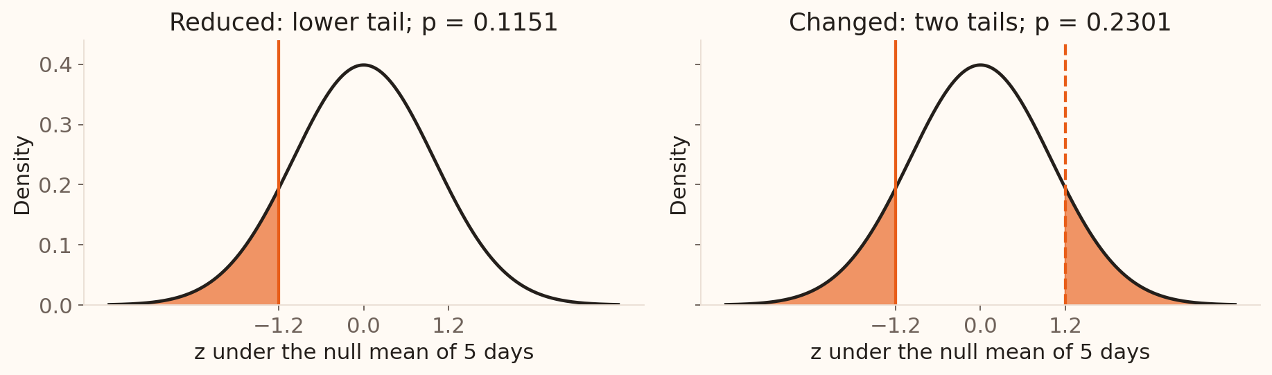
Alternative	Probability under the null	p-value
\(\mu<5\)	\(P(Z\le-1.20)\)	0.1151
\(\mu\ne5\)	\(P(|Z|\ge1.20)\)	0.2301

Use the Week 4 cumulative normal table: Phi(1.20)=0.8849, so Phi(−1.20)=0.1151. Under a symmetric continuous null distribution, the matching two-sided p-value is twice the smaller one-tail area. That doubling rule is not universal for every possible test. Ask students which picture matches the word changed and which matches reduced.

Approval times: compare both approaches

Our observed statistic is \(z=-1.20\). Use \(\alpha=0.05\).

Planned question	Critical-value check	P-value check	Decision
Has the mean fallen?	\(-1.20>-1.645\)	\(0.1151>0.05\)	Fail to reject
Has the mean changed?	\(-1.960<-1.20<1.960\)	\(0.2301>0.05\)	Fail to reject

The two approaches agree for each planned question.

Conclusion for the planned decrease: the estimated mean is 0.3 days lower, with insufficient evidence of a lower population mean at the 5% level.

Allow two minutes. For the lower-tail question, sample means at or below 4.7 days would occur about 11.5% of the time if the population mean were 5 days under the stated model. The observed difference is therefore not sufficiently unusual to reject at 5%. The two-sided p-value accounts for equally extreme differences on either side of 5. Both full p-values are compared with alpha=0.05. Failing to reject does not establish equality or absence of a useful effect. Report the observed difference and its uncertainty alongside the decision.

What changes when the SD is estimated?

Suppose 1.5 days is the sample SD \(s\), rather than a known population SD.

\[t=\frac{4.7-5}{1.5/\sqrt{36}}=-1.20,\qquad df=35.\]

Quantity	Known \(\sigma\): normal	Estimated \(\sigma\): t with 35 df
Lower-tail p-value	0.1151	0.1191
Lower critical value at 5%	−1.645	−1.690

The numerical statistic stays the same; the reference distribution changes.

Exact t inference assumes independent normal observations; otherwise judge the approximation. Calculations use unrounded quantiles. The critical value is −1.68957, or −1.690 to three decimals. The t distribution is the standard choice when sigma is estimated; the nearby normal values illustrate the large-sample shortcut from the earlier guide. Session 6 applies the t method to the skewed balance sample and to paired differences.

Confidence interval versus hypothesis test

Aspect	Confidence interval	Hypothesis test
Question	Which parameter values are plausible?	Is there evidence against a specified claim?
Result	A range with a confidence level	A test statistic, p-value and decision
Chosen level	For example, 95% confidence	For example, 5% significance
Approval-time example	Mean time: 4.21–5.19 days	Test \(\mu=5\): two-sided \(p=0.2301\)

The interval shows the size and uncertainty of the effect; the test assesses a specified benchmark.

Allow two minutes. Both methods use the same sample information and a sampling model. Confidence refers to repeated-sampling coverage, not a 95% probability assigned to a fixed parameter after observing the data. A test provides a statistical decision at the chosen level; it does not prove the null or alternative true. Intervals can be one-sided or two-sided, as can tests. The numerical example uses known sigma=1.5, n=36, mean=4.7 and the same normal model as the preceding two-sided test. For a matching pair of procedures, the interval and test can express the same evidence in different ways.

Use a confidence interval to test a mean

For \(H_0:\mu=5\) versus \(H_A:\mu\ne5\) at 5% significance, calculate the matching 95% confidence interval:

\[4.7\pm1.96(0.25)=\boxed{(4.21,\ 5.19)\text{ days}}.\]

Where is the null value?	Decision using the interval
Outside the interval	Reject \(H_0\).
Inside the interval	Fail to reject \(H_0\).

5 days lies inside, so fail to reject \(H_0\): the same decision as the two-sided test with \(p=0.2301\).

Allow two minutes. A confidence interval can be used to test a hypothesis: for matching mean z or t procedures, a two-sided level-alpha test rejects null values outside its (1−alpha) confidence interval. The same inequality can be read as a test of mu0 or as an interval for mu. Use unrounded critical values in computation; the displayed interval uses the familiar rounded 1.96. At an exact endpoint, use the same equality convention in both procedures; in a continuous model that boundary event has probability zero.

Match the confidence level, direction, assumptions and reference distribution. A one-sided 5% test uses a one-sided 95% confidence bound. The two-sided 95% interval here addresses changed, rather than the separate question of a decrease. For a proportion, the interval must be obtained by inverting the same test for exact agreement of the decision rules; the Wald interval and a null-SE z-test can differ near the boundary. Session 6 applies this distinction to a balance example with different one-sided and two-sided decisions.

Testing a Proportion

Case: default-rate threshold

The UCI credit dataset records 6,636 next-month defaults among 30,000 accounts:

\[\hat p=6636/30000=0.2212.\]

Use 20% as a teaching risk-monitoring threshold.

Could sampling variation under a 20% default model plausibly explain the observed 22.12%?

Source: Yeh, UCI Default of Credit Card Clients. The 20% threshold is illustrative, not a published policy limit.

Why the test uses \(p_0\) in its standard error

Week 4 gave \(SE(\hat p)=\sqrt{p(1-p)/n}\) under independent Bernoulli sampling.

Task	Rate used in the standard error
Estimate an unknown rate with an interval	\(\hat p\): estimate the unknown variability
Test a specified rate \(H_0:p=p_0\)	\(p_0\): calculate variability under the null

For \(p_0=0.20\) and \(n=30{,}000\), check \(np_0=6{,}000\) and \(n(1-p_0)=24{,}000\).

Both expected counts exceed 10, supporting the normal approximation under the independence model. This explains the change from the interval formula instead of asking students to memorise two denominators. An interval produced by inverting this null-SE test is the Wilson score interval; the introductory Wald interval uses a different construction. Consequently their borderline decisions need not match exactly. Session 6 examines an approximate versus exact binomial result.

Testing a default-rate benchmark

Hypothesis	Role
\(H_0:p=0.20\)	Benchmark model used for calculation
\(H_A:p>0.20\)	Direction of the suspected departure

\[z=\frac{\hat p-p_0}{\sqrt{p_0(1-p_0)/n}} =\frac{0.2212-0.20}{\sqrt{0.20(0.80)/30000}}=9.18.\]

The observed proportion is 9.18 null standard errors above the benchmark.

For the one-sided question, the broader null is p at most 0.20. The test is calibrated at its boundary p=0.20. The empirical records are used to demonstrate the calculation under an independent Bernoulli model; the public dataset does not itself establish representative sampling from all customers.

Default-rate test: calculate the tail probability

For the one-sided alternative,

\[p\text{-value}=P(Z\ge9.18\mid H_0)\approx2.2\times10^{-20}.\]

Under the benchmark model, a proportion at least this high would be extraordinarily unusual.

The p-value is the probability, assuming the null model and its conditions, of obtaining a test statistic at least as extreme in the direction specified by the alternative. It is not the probability that H0 is true, the probability that chance caused the finding, or the size of the effect.

Default-rate test: report the finding

Result	Statistical decision
\(p\le\alpha\)	Reject \(H_0\)
\(p>\alpha\)	Fail to reject \(H_0\)

With \(p\ll0.05\), reject \(H_0\). The practical difference is 2.12 percentage points.

“Fail to reject” is not “prove true”.

Because the 30,000 records are the published dataset rather than a documented probability sample, the p-value is model-based. The observed 22.12% remains descriptive fact for this dataset.

Read a p-value correctly

A prespecified test gives p = 0.03. What does this mean under the test assumptions?

1. The null hypothesis has a 3% chance of being true
2. Under the null, a statistic at least as extreme has probability 3%
3. The effect is 3%
4. The study is correct with probability 97%

Format: multiple choice, one answer; 90 seconds. Correct: option 2. Ask students to identify the conditioning assumption and the meaning of at least as extreme for a one-sided or two-sided alternative.

When it comes to real data

Start with the research question and the observational unit.

Step	What should you establish?
Understand the data	Target population, sample size, missing values, repeated observations and distribution shape.
State the hypotheses	Mean or proportion? What benchmark? One or two tails? Choose \(\alpha\) in advance.
Choose and calculate	Mean: \(z\) if \(\sigma\) is known, otherwise \(t\). Proportion: check counts before a normal approximation.
Make the comparison	Statistic versus critical value; p-value versus \(\alpha\); or null value versus a matching confidence interval.
Report in context	Estimate, interval, p-value, decision, assumptions and practical importance.

Allow three minutes as the transition from worked summaries to independent analysis. Identify what one row represents and how the data relate to the target population. Check missingness, skewness, extremes and dependence; repeated measurements of one customer do not automatically give independent observations. State the parameter, benchmark, direction and significance level before inspecting outcome comparisons. If the question was suggested by the data, label the analysis exploratory.

Use a mean procedure for numerical outcomes and a proportion procedure for binary outcomes. For a mean, estimate sigma with s when it is unknown and use the t reference, with the large-sample normal shortcut understood as an approximation. For a proportion test, check expected successes and failures using the null rate. With small counts, consider an appropriate binomial method. Compare a statistic to a critical value on the same scale, and a p-value to alpha. The confidence-interval approach requires a matching level and direction. Select the method before seeing whether it gives the preferred decision.

Return to the examples: balance is numerical, so the sample SD leads to a t procedure; default is binary, so the proportion test uses the null-rate standard error. Report the estimated difference in days, currency or percentage points as appropriate. A small p-value alone does not establish practical importance, representative sampling or causality. The next session uses real records to practise these choices, including an exact-versus-approximate comparison and paired observations.

Session 5 takeaway

• Judge an estimator by its bias, precision and behaviour as the sample grows.
• Build an interval from an estimate, standard error and critical value.
• Confidence describes repeated-sampling coverage.
• Recognise false alarms and missed signals when making testing decisions.
• Use critical values, p-values or a matching interval to assess a planned hypothesis.
• Report the estimated effect, uncertainty and practical meaning.

Next: apply these procedures to real data and paired differences, then examine errors, power and practical consequences.