Introduction to Hypothesis Testing
Example: Milk
A dairy company suspects that some suppliers are adding water to their milk. This can be detected by checking the freezing point of the milk.
The freezing temperature of natural milk is normally distributed, with
Added water raises the freezing temperature towards 0°C, the freezing point of water.
A random sample of 16 lots produces the sample mean of -0.514°C.
Question: Are the suppliers honest?
Calculations
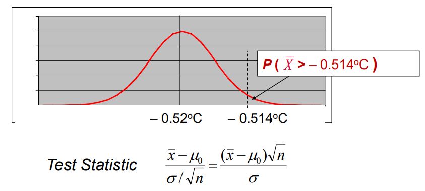
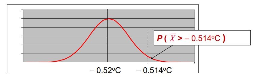
Calculate the probability of getting a sample mean of -0.51 or larger:
- Sampling distribution of \(\bar{X}\) under \(H_0\) \[\bar{X} \sim N (-0.52, 0.01^2 / n)\]
Calculations
In this example:
We call the probability of getting a sample mean that far from the prescribed population mean or even further as p-value.
\[\begin{aligned}
\mathbb{P}(\bar{X} > -0.514) & = \mathbb{P}( \frac{\bar{X} - \mu}{SE} > \frac{-0.514 - \mu}{SE}) \\
&= \mathbb{P}( Z > \frac{-0.514 - (-0.52)}{0.0025}) \\
&= \mathbb{P}( Z > 2.4) \\
&= 0.0082
\end{aligned}\]
What does mean of this 0.0082?
\(\mathbb{P}(\bar{X} > -0.514) = 0.0082\)
The probability that we get this worse sample mean just due to the sampling (we’re so unlucky) is very small
For a normal distribution, lower than 5% (or less) can be considered an "unlikely" case (can be ignored)
However, something unlikely to happen, but it indeed happened
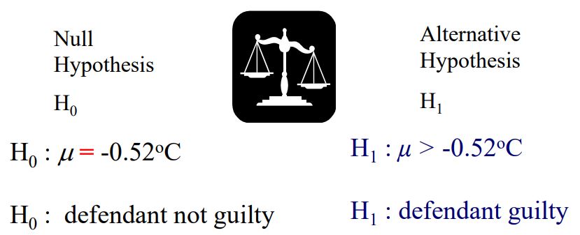
It is very likely that the null hypothesis (\(H_0\)) is incorrect (contradiction)
in favour of the alternative hypothesis, defendant guilty!
Hypothesis Testing
Hypothesis testing can be used to determine whether a statement about the value of a population parameter should or should not be rejected.
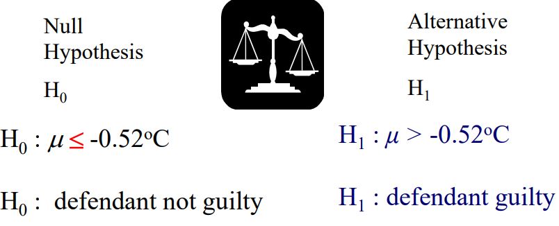
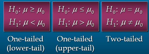
The null hypothesis, denoted by \(H_0\), is a tentative assumption about a population parameter.
The alternative hypothesis, denoted by \(H_1\), is the opposite of what is stated in the null hypothesis.
The alternative hypothesis is often what the test is attempting to establish (one side or two sides).
Another key concept in hypothesis testing: significance level, denoted as \(\alpha\).
Everyone can make a mistake
In reality, the event with a small probability can still happen:
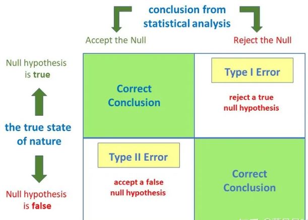
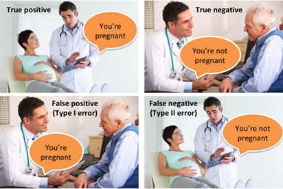
The hypothesis is true, but due to ignoring the chance of extreme events happening, we incorrectly reject the hypothesis.
The hypothesis is false, but due to ignoring the chance of extreme events happening, we incorrectly accept the hypothesis.
Both errors can happen:
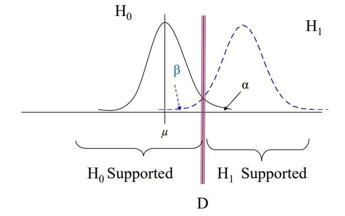
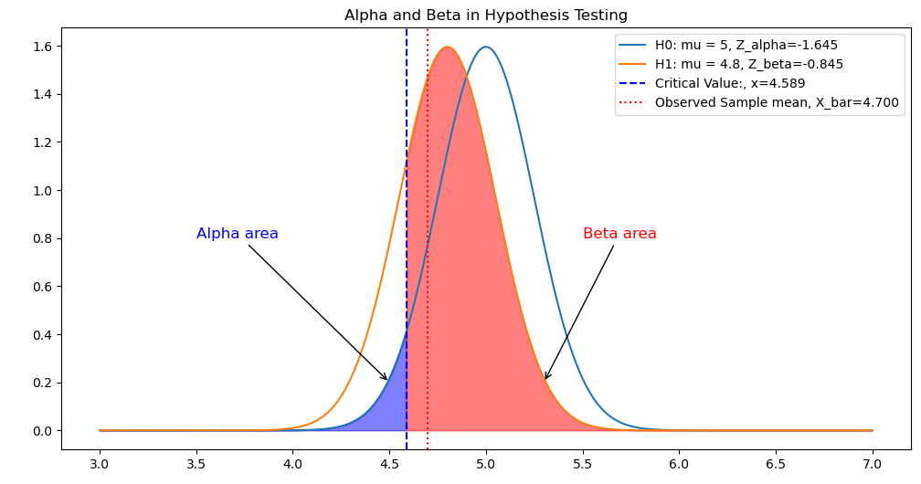
The error in the first scenario is called a Type I error, denoted as alpha, which is what we refer to as the significance level (\(\alpha\)).
The error in the second scenario is called a Type II error, generally denoted as \(\beta\).
Everyone can make a mistake
In the case of a Type 1 error, we are considering whether the sample data occurs in the extreme cases within the assumed population. If the answer is ‘YES’, it means that the original hypothesis is correct, but after all our hard work, we happen to fall into the situation where an error occurs, leading to an incorrect conclusion.
In the case of a Type 2 error, we are considering whether the sample data happens to be included when the population hypothesis is incorrect. If the answer is ‘YES’, it means that the original hypothesis is wrong, but due to an unfortunate coincidence, this error is supported by the information calculated from the sample data, leading us to make an incorrect conclusion.
Deciding Between \(H_0\) and \(H_1\)
Note: this is a one-talied test, since the rejection region occupies only one side of the distribution
Steps of Hypothesis Testing
Step 1: Develop the null and alternative hypotheses (upper or lower or two sides!). For example, testing for mean:
Step 2: Specify the level of significance \(\alpha\) and the test statistic
Step 3: Collect the sample data and compute the test statistic
Then we have two approaches to making decisions:
Steps of Hypothesis Testing: p-Value Approach
Steps of Hypothesis Testing: Critical Value Approach
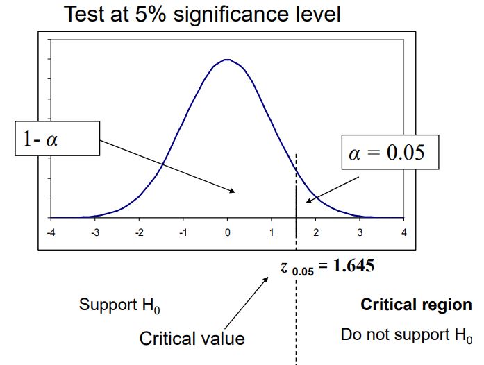
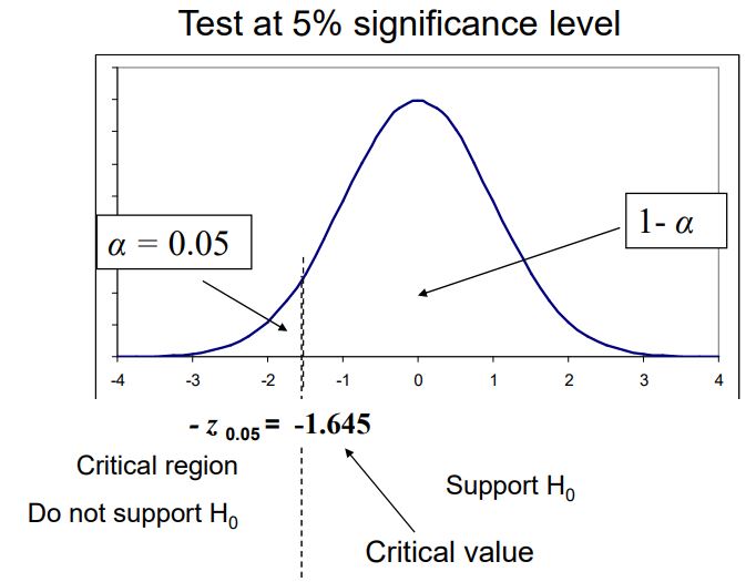
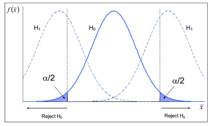
Step 4: Use the level of significance (\(\alpha\)) to determine the critical value and the rejection rule.
Step 5. Use the value of the test statistic and the rejection rule to determine whether to reject \(H_0\).
Lower tail: Reject \(H_0\) if \(z \leq -z_{\alpha}\)
Upper tail: Reject \(H_0\) if \(z \geq z_{\alpha}\)
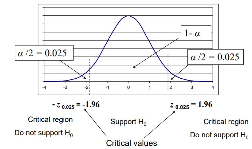
Two tails: Reject \(H_0\) if \(z \geq z_{\alpha/2}\) or \(z \leq -z_{\alpha/2}\)
Critical region for \(H_1: \mu > K\)
Critical region for \(H_1: \mu < K\)
How to do Hypothesis Test
Scenario
Role: Risk Analyst at a bank
Objective: Evaluate the impact of a new credit approval system on the average loan approval time.
Historical Average: \(5\) days
Known Standard Deviation: \(1.5\) days
Sample Data: \(36\) loan applications
Sample Mean: \(4.7\) days
Hypothesis and Statistic
Null Hypothesis (\(H_0\)): \(\mu = 5\) (No change in average approval time)
Alternative Hypothesis (\(H_1\)): \(\mu \neq 5\) (Change in average approval time)
Choose a significance level (\(\alpha\)) of \(5\%\).
Using Z-statistic (known population standard deviation): \[Z = \frac{( \bar{x} - \mu )}{\frac{\sigma}{\sqrt{n}}}\]
\(\bar{x} = 4.7\), \(\mu = 5\), \(\sigma = 1.5\), \(n = 36\) \[Z = \frac{( 4.7 - 5 )}{\frac{1.5}{\sqrt{36}}} = -1.2\]
P-Value Approach
The p-value for \(Z = -1.2\) is approximately \(0.23\)
\(p > \alpha\) (\(0.23 > 0.05\))
Fail to reject \(H_0\)
Insufficient evidence to conclude that the average loan approval time has changed.
Critical Value Approach
Critical Z-value for \(\alpha = 0.05\) in a two-tailed test: \(\pm 1.96\)
Calculated \(Z = -1.2\) doesn’t fall in the critical region \((-\infty, -1.96) \cup (1.96, \infty)\)
Fail to reject \(H_0\)
Insufficient evidence to conclude that the average loan approval time has changed.
Scenario II
Role: Risk Analyst at a bank
Objective: Evaluate the impact of a new credit approval system on the average loan approval time.
Historical Average: \(5\) days
Known Standard Deviation: \(1.5\) days
Sample Data: \(36\) loan applications
Sample Mean: \(4.7\) days
Now, our question is to check if the new credit approval system reduces the approval time.
Hypothesis and Statistic II
Null Hypothesis (\(H_0\)): \(\mu \geq 5\) (No reduction in average approval time)
Alternative Hypothesis (\(H_1\)): \(\mu < 5\) (Reduction in average approval time)
Choose a significance level (\(\alpha\)) of \(0.05\).
Using Z-statistic (known population standard deviation): \[Z = \frac{( \bar{x} - \mu )}{\frac{\sigma}{\sqrt{n}}}\]
\(\bar{x} = 4.7\), \(\mu = 5\), \(\sigma = 1.5\), \(n = 36\) \[Z = \frac{( 4.7 - 5 )}{\frac{1.5}{\sqrt{36}}} = -1.2\]
Solution II
P-Value Approach:
Critical Value Approach:
Therefore, insufficient evidence to conclude that the average loan approval time has been reduced.
Scenario III: unknown standard deviation \(\sigma\)
Role: Risk Analyst at a bank
Objective: Evaluate if the new credit approval system reduces the average loan approval time.
Historical Average: \(5\) days
Sample Data: \(36\) loan applications
Sample Mean: \(4.7\) days
Sample Standard Deviation: \(1.5\) days
Hypothesis and Test Statistic III
Null Hypothesis (\(H_0\)): \(\mu \geq 5\) (No reduction in average approval time)
Alternative Hypothesis (\(H_1\)): \(\mu < 5\) (Reduction in average approval time)
Choose a significance level (\(\alpha\)) of \(0.05\).
Using t-statistic (unknown population standard deviation): \[t = \frac{( \bar{x} - \mu )}{\frac{s}{\sqrt{n}}}\]
\(\bar{x} = 4.7\), \(\mu = 5\), \(s = 1.5\), \(n = 36\) \[t = \frac{( 4.7 - 5 )}{\frac{1.5}{\sqrt{36}}} = -1.2\]
Solution III
Critical Value Approach:
Degrees of Freedom = \(n - 1 = 35\)
Critical t-value for \(\alpha = 0.05\) and \(35\) df: \(-1.689\)
Calculated \(t = -1.2\) is greater than \(-1.689\)
Fail to reject \(H_0\)
P-Value Approach:
Therefore, insufficient evidence to conclude that the average loan approval time has reduced.
Sample Size for Test
In terms of population mean (both estimator and test),
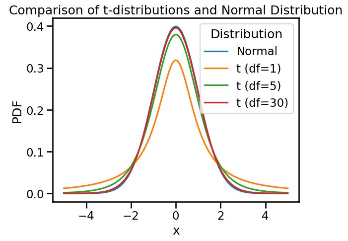
If \(\sigma\) is unknown, you need to use t-distribution to make an inference
Since t-distribution with a degree of freedom greater than 30 is already quite similar to a normal distribution, we can also just use the normal distribution to make inferences in the cases (unknown \(\sigma\))
One-side or Two-side test?
Direction: Area of Concerns
Clue Words: Faster, Improving, Slower, Getting Worse, Recession, Fall in Trade etc.
Hints:
IF there is a Direction/ Area of concern, then ONE-TAIL(ONE-SIDE)
If NOT, then TWO-TAIL (TWO-SIDE)
Scenario IV: Customer Satisfaction in Banking
Historical proportion of satisfied customers: \(p = 0.7\)
After one year of hard work on customer satisfaction, we have
Sample proportion of satisfied customers (\(\hat{p}\)): \(0.75\)
Sample size (\(n\)): \(100\)
Hypothesis and Test Statistic IV
Null Hypothesis \(H_0\): \(p \leq 0.7\) (no positive change)
Alternative Hypothesis \(H_1\): \(p > 0.7\)
Choose a significance level (\(\alpha\)) of \(0.05\).
Recap: \[z = \frac{\hat{p} - p}{\sqrt{\frac{p(1-p)}{n}}}\] Did you still remember the conditions?
np > 5 or 10
n(1-p) > 5 or 10
\(\hat{p} = 0.75\), \(p = 0.7\), \(n = 100\)
\(z = \frac{0.75 - 0.7}{\sqrt{\frac{0.7 \times 0.3}{100}}} = 1.16\)
Solution IV
Critical Value Approach:
P-Value Approach:
Therefore, insufficient evidence to conclude that the proportion of satisfied customers has positively increased.
Scenario IV+
To reject the null hypothesis, what is the minimum sampling proportion we have to observe? \[z = \frac{\hat{p} - 0.7}{\sqrt{\frac{0.7 \times 0.3}{100}}} > 1.645\]
Therefore: \[\hat{p} > 0.775\]