Statistics for Analytics

Session 6: One-Sample & Paired Inference

Dr Zexun Chen

Zexun.Chen@ed.ac.uk

Today’s route

Choose the observational unit, test the claim and report the size and uncertainty of the effect.

Teaching time: 110 minutes, plus a 10-minute break. The timed blocks include calculation, discussion and Wooclap debriefs.

• 000–005 min: Retrieve the testing logic
• 005–035 min: Apply one-sample procedures; compare approximate and exact proportion results
• 035–055 min: Paired differences and the unit-of-analysis activity
• 055–065 min: Break
• 065–090 min: Error costs, power and detection planning
• 090–115 min: Apply interval/test decisions in the reporting workshop; practical-importance activity
• 115–120 min: Synthesis and questions

Reference slides are available after the session takeaway and are not part of the core two-hour route.

One-Sample Procedures

From a benchmark to a procedure

Session 5 constructed confidence intervals and carried out one-sample z and t tests.

Today we apply that workflow to real records, then analyse paired changes and the consequences of testing errors.

Question	Parameter
Has mean balance increased?	Mean balance \(\mu\)
Has the subscription rate fallen?	Proportion \(p\)
Have the same clients’ bills changed?	Mean within-client difference \(\mu_d\)

Choose the parameter and the observational unit before calculating.

Five-minute retrieval. Ask what is assumed when calculating a p-value and what a rejection means. Students should connect the parameter to the question. Explain that the paired analysis reuses the one-sample t procedure after constructing differences.

Practice: plan the balance test

The Week 5 sample gave

\[n=400,\qquad\bar x=€1{,}517.92,\qquad s=€2{,}842.26.\]

The planned question is whether the mean balance exceeds €1,250.

1. State the null and alternative hypotheses.
2. Choose the reference distribution and standard error.
3. Predict which tail supplies the p-value.

UCI Bank Marketing; sample seed 11624. The benchmark is illustrative.

Allow four minutes before the solution. Students now apply Session 5’s workflow: broader null mu≤1250, alternative mu>1250, calculation at the boundary, t with 399 df and SE s/sqrt(n). The right tail corresponds to the prespecified increase. Ask them to retrieve the 95% interval, €1238.53 to €1797.30, without treating a two-sided interval as the match to a one-sided 5% test; the reporting workshop resolves that distinction.

Balance test: choose the sampling model

The population SD is estimated from the sample, so use

\[t=\frac{\bar x-\mu_0}{s/\sqrt n},\qquad df=n-1=399.\]

Check: random selection, the sampling fraction, balance skewness and extreme observations.

This is application of the t procedure developed in Session 5. Balances are strongly skewed; the t reference is a large-sample approximation here, not an exact small-normal-sample result. The target remains the 45,211-record published frame. The finite population multiplier is about 0.9956 and is omitted in these examples. A historical estimate of SD is not automatically a known sigma.

Real balance sample

A reproducible sample from the bank campaign records gives

\[n=400,\quad\bar x=€1517.92,\quad s=€2842.26.\]

Test \(H_0:\mu=€1250\) versus \(H_A:\mu>€1250\).

\[t=\frac{1517.92-1250}{2842.26/\sqrt{400}}=1.89,\quad df=399.\]

Source: UCI Bank Marketing; sample seed 11624. The €1,250 benchmark is illustrative.

Balance-test conclusion

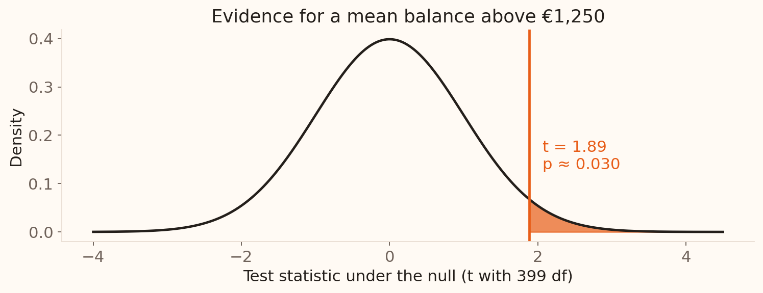
Conclusion: the approximate test supports a mean above €1,250. The estimated excess is €267.92.

The t reference is approximate for these strongly skewed balances. The 400-record random sample supports inference to the finite published frame under the earlier sampling assumptions. Report the estimate and uncertainty as well as the decision.

Campaign-rate example

In the reproducible sample of 400 campaign records, 30 clients subscribed. Compare with a 10% historical benchmark.

Test \(H_0:p\ge0.10\) versus \(H_A:p<0.10\).

\[\hat p=30/400=0.075\]

\[z=\frac{0.075-0.10}{\sqrt{0.10(0.90)/400}}=-1.67.\]

For \(H_A:p<0.10\), \(p\approx0.048\).

The estimated shortfall is 2.5 percentage points; the approximate result is close to the 5% threshold.

Source: UCI Bank Marketing; sample seed 11624. The 10% benchmark is illustrative.

Use the boundary null p0=0.10. Its expected counts are 400×0.10=40 subscribers and 400×0.90=360 non-subscribers; both exceed 10. The standard error uses the null rate, under independent Bernoulli sampling. This is a normal-approximation z-test. The exact lower-tail binomial probability is 0.0524, so this borderline example changes its reject/fail-to-reject label with the approximation. Keep the estimated rate and practical shortfall central to the interpretation and report the method used.

The same count: approximate or exact?

Under \(H_0:p=0.10\), the subscription count satisfies \(X\sim\operatorname{Bin}(400,0.10)\).

Method for the planned decrease	Lower-tail probability	Decision at 5%
Normal z approximation	0.0478	Reject
Exact binomial: \(P(X\le30)\)	0.0524	Fail to reject

The estimate is 7.5% under either method, a shortfall of 2.5 percentage points.

Allow five minutes for comparison and discussion. Reuse Week 4’s binomial-to-normal approximation ideas: adequate expected counts do not make the approximation exact, and small numerical differences matter near a threshold. The binomial result assumes independent Bernoulli observations with common p. For inference conditional on a fixed finite frame with sampling without replacement, the exact count model would instead be hypergeometric. Here both rows use the same Bernoulli process model to isolate approximation error.

Campaign rate: report the method and the evidence

“The observed subscription rate was 7.5%, compared with the 10% benchmark. The exact lower-tail binomial test gave p = 0.0524, which exceeds the prespecified 5% level.”

What additional information would help assess whether the 2.5-point shortfall warrants action?

Use the remaining one-sample block for a brief report discussion. Students should ask about precision, customer selection, historical comparability, campaign costs and the practical threshold. State which test was used. The difference between 0.0478 and 0.0524 should not drive a large change in the substantive claim. The process model is an assumption for this exercise; the published records are not evidence of representative sampling from future customers. Model-based inference and a finite-frame description answer different questions.

Paired Differences

When data are paired

Repeated measures

Before and after on the same unit

Natural matching

Matched branches with similar portfolios

Pairing is useful when members of a pair are similar.

Choose the unit of analysis

The same 150 borrowers have August and September bills. Which analysis addresses their mean monthly change?

1. An independent test with 300 observations
2. A paired analysis of 150 within-borrower differences
3. A two-proportion test
4. Treat every bill as an independent borrower

Format: multiple choice, one answer; 60 seconds. Correct: option 2. Debrief: sample size is the number of complete pairs, and the SD needed is the SD of the differences. Independence is required between borrowers, not within each pair.

Analyse within-pair differences

For each complete pair, define \(d_i=x_{i,\text{after}}-x_{i,\text{before}}\).

Then perform a one-sample t procedure on \(d_1,\ldots,d_n\).

Task	Calculation
Confidence interval	\(\bar d\pm t^*_{n-1}s_d/\sqrt n\)
Test \(H_0:\mu_d=0\)	\(t=\bar d/(s_d/\sqrt n)\), with \(df=n-1\)

The sample size is the number of complete pairs; \(s_d\) is the SD of their differences.

The same clients in two months

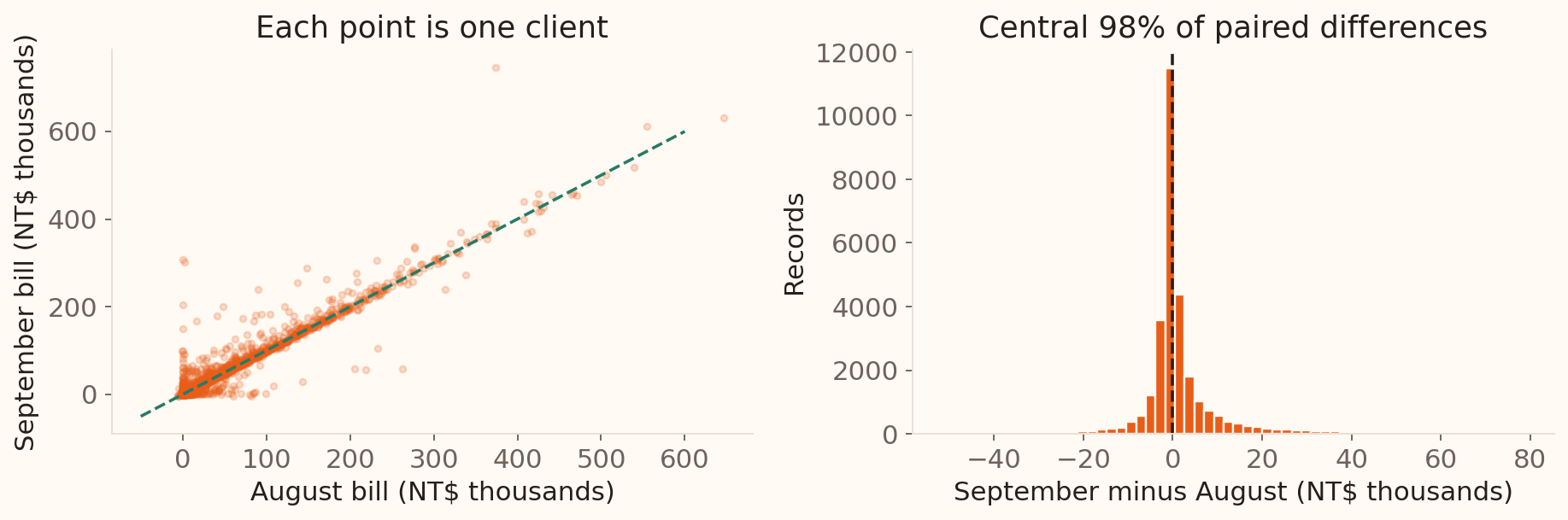
The comparison uses each client’s change, preserving the link between their two bills.

UCI Default of Credit Card Clients. Scatter: 2,500 sampled clients; histogram: central 98% of differences. Calculations use all 30,000 pairs.

Paired monthly bills

For the same 30,000 accounts, define \(d=\) September bill − August bill.

\[\bar d=2044.26\ \mathrm{NTD},\quad s_d=22684.89\ \mathrm{NTD}.\]

\[t=15.61,\quad df=29{,}999,\]

with a 95% interval of 1,788 to 2,301 NTD for the mean within-record change.

Source: UCI Default of Credit Card Clients, BILL_AMT1 and BILL_AMT2. Time dependence and collection context limit wider inference.

Errors & Power

Truth table: false alarms, missed signals and power

A risk team tests whether the default rate exceeds 20%. Compare two possible population rates.

Our decision	True rate is 20%	True rate is 22%
Reject \(H_0\)	Type I: false alarm, probability \(\alpha\)	Correct detection, probability \(1-\beta\)
Fail to reject \(H_0\)	Correct decision, probability \(1-\alpha\)	Type II: missed increase, probability \(\beta\)

Power \(=1-\beta\) is the probability of detecting the specified increase to 22%.

Choosing \(\alpha=0.05\) does not set \(\beta\): detection also depends on sample size, variability and the true change.

Allow four minutes. The planned hypotheses are H0:p≤0.20 and HA:p>0.20. Read each column as a different population state, then ask how repeated samples could lead to either decision. For this table, consider a test calibrated to have false-alarm probability alpha at the boundary p=0.20. The probability of a correct non-rejection there is 1−alpha. At the specified alternative p=0.22, beta is the probability of failing to reject, and power 1−beta is the probability of detection. For other true rates, beta and power change.

A level-alpha procedure controls Type I probability at or below alpha across the null. In a discrete binomial test the achieved boundary probability may be below the nominal level; the following figure uses a continuous normal approximation to make the power comparison visible. Alpha and beta are conditional probabilities of decisions under specified population states, not probabilities assigned to H0 after seeing the data. Connect the cells to the false-alarm and missed-signal costs on the next slide.

Which error is more costly here?

A risk team tests whether the portfolio default rate exceeds its benchmark.

• A false alarm triggers an expensive review.
• A missed increase delays action on a deteriorating portfolio.

Discuss how lowering the significance level changes these risks at a fixed sample size. How could the team improve detection without increasing the false-alarm rate?

Allow eight minutes for the operational-cost discussion. Together with four minutes for the truth table, this leaves thirteen minutes in the block to compare power at the two sample sizes and discuss practical effect sizes. Lower alpha reduces Type I risk but generally increases Type II risk for a specified alternative at fixed n. A larger well-designed sample improves power while keeping alpha fixed. Explain that alpha alone is not an operational loss function; costs, effect size and the response to an alarm matter. The following power figure shows the role of n.

What increases power?

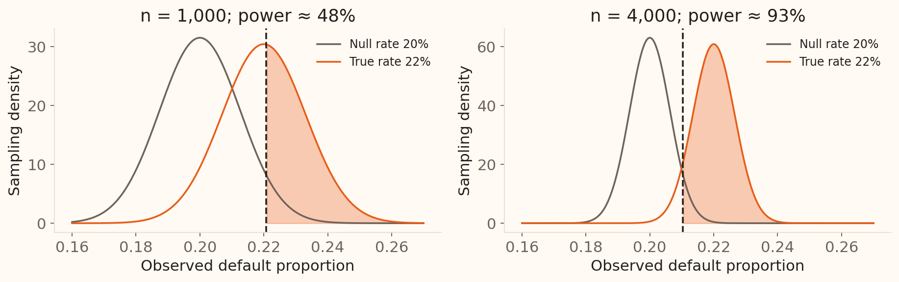
Larger samples, larger effects, and lower variability improve power. Raising \(\alpha\) also increases false alarms.

Illustrative normal approximations: one-sided test at \(\alpha=0.05\), null rate 0.20, alternative rate 0.22. Orange shaded area is power.

Significance is not importance

Question	Tool
Is evidence inconsistent with \(H_0\)?	p-value
How large is the effect?	Point estimate
How precise is it?	Confidence interval
Does it matter operationally?	Domain threshold

A good report answers all four.

Reporting Evidence

The same sample, two planned questions

The balance sample gives \(t=1.885\) against €1,250, with \(df=399\).

Planned alternative	p-value
Mean above €1,250	0.030
Mean different from €1,250	?

The matching two-sided 95% interval is €1,238.53 to €1,797.30.

Explain the two decisions at 5% and their agreement with the interval.

Allow 15 minutes of the reporting workshop: 5 minutes in pairs, 5 minutes comparing explanations and 5 minutes building a model report. The two-sided p-value is about 0.0601, so it fails to reject at 5%; 1250 is inside the two-sided interval. The prespecified one-sided p=0.0301 supports an increase under the approximate t model. It is compared with a matching one-sided confidence bound, not this two-sided 95% interval. Students must not choose the direction after seeing the data. Report estimated increase €267.92, sampling scope, skew and the approximate method. The practical-importance activity and discussion use the remaining 10 minutes of this block.

Would this change a risk decision?

A portfolio test gives p = 0.03, but the estimated reduction in default is only 0.1 percentage point. What can you conclude, and what else would you need before acting?

Format: open response; two minutes in pairs, then collect responses. Expected: evidence against the specified null at 5% under the model; effect size and confidence interval, intervention cost, error costs, study design, and whether the comparison supports causality. Do not infer operational value from the p-value alone.

Session 6 takeaway

• Use one-sample procedures for a mean, a proportion or paired differences.
• Choose the direction of a test before seeing its result.
• Distinguish false alarms, missed signals and practical importance.
• Report the effect, interval, assumptions and conclusion together.

Next: compare independent groups and categorical outcomes.

Reference

Pairing reduces noise

\[\operatorname{Var}(X-Y)= \operatorname{Var}(X)+\operatorname{Var}(Y)-2\operatorname{Cov}(X,Y)\]

Positive within-pair correlation reduces variation in differences and can improve precision.

Keep the pairs intact: analysing the two columns as independent groups uses a different standard error.

The paired t procedure needs independence between pairs and a suitable distribution of the differences. It does not need the two measurements within a pair to be independent. With positive within-pair association, preserving pairing typically improves precision. A before/after difference alone does not establish a causal effect of an intervention.

Multiple testing

If 20 independent true null hypotheses are tested at \(\alpha=0.05\),

\[P(\text{at least one false positive})=1-0.95^{20}\approx0.64.\]

Pre-specify primary outcomes and adjust when many comparisons are explored.