CMSE11624 Statistics for Analytics

Session 7: Testing for Two Populations

Dr Zexun Chen

Zexun.Chen@ed.ac.uk

Table of Contents

Two Population Means: Independent Samples

Motivation Example

Problem

• You are a data analyst in the UK’s banking sector.

• The management team wants to know if there’s a significant difference in loan approval times between Lloyds Bank and HSBC.

image

Notes

• Population variances may be known or unknown, equal or unequal

• Sample sizes may not be the same

Inferences About Difference Between Two Population Means: \(\sigma_1\) and \(\sigma_2\) Known

• Interval Estimation of \(\mu_1 -\mu_2\)

• Hypothesis Tests about \(\mu_1 -\mu_2\)

Comparison of Two Population Means: Estimation

• Let \(\mu_1\) equal the mean of population 1 and \(\mu_2\) equal the mean of population 2.

• The difference between the two population means is \(\mu_1 - \mu_2\).

• To estimate \(\mu_1 - \mu_2\), we will select a simple random sample of size \(n_1\) from population 1 and a simple random sample of size \(n_2\) from population 2.

• Let \(\bar{x}_1\) equal the mean of sample 1 and \(\bar{x}_2\) equal the mean of sample 2.

• The point estimator of the difference between the means of the populations 1 and 2 is \(\bar{x}_1 - \bar{x}_2\).

Sampling Distribution of \(\bar{x}_1 - \bar{x}_2\)

• Expected Value: \[E(\bar{x}_1 - \bar{x}_2) = \mu_1 - \mu_2\]

• Standard Deviation (Standard Error): \[\sigma_{\bar{x}_1-\bar{x}_2} = \sqrt{\frac{\sigma_1^2}{n_1} + \frac{\sigma_2^2}{n_2}}\]

• where:

  • \(\sigma_1 =\) standard deviation of population 1

  • \(\sigma_2 =\) standard deviation of population 2

  • \(n_1 =\) sample size from population 1

  • \(n_2 =\) sample size from population 2

• Interval Estimate: \[\bar{x}_1 - \bar{x}_2 \pm z_{\alpha/2} \sqrt{\frac{\sigma_1^2}{n_1} + \frac{\sigma_2^2}{n_2}}\]

• where: \[1 - \alpha \text{ is the confidence coefficient}\]

Scenario I: Estimation

Data (the figures here are not the facts):

• Lloyds Bank: A random sample of 50 loan applications

  • Average approval time of 7 days.

  • Known standard deviation of 2 days.

• HSBC: A random sample of 60 loan applications

  • Average approval time of 6.5 days.

  • Known standard deviation of 2.5 days.

Task:

• Get the 95% confidence interval of the differences in loan application processing time between Lloyds and HSBC bank.

Solution I-E

\[\begin{aligned} \text{For Lloyds Bank (LB):} & \quad n_{LB} = 50, \bar{x}_{LB} = 7, \sigma_{LB} = 2 \\ \text{For HSBC Bank:} & \quad n_{HSBC} = 60, \bar{x}_{HSBC} = 6.5, \sigma_{HSBC} = 2.5 \end{aligned}\]

The formula for the 95% confidence interval is: \[CI = \bar{x}_{LB} - \bar{x}_{HSBC} \pm z_{\alpha/2} \sqrt{\frac{\sigma_{LB}^2}{n_{LB}} + \frac{\sigma_{HSBC}^2}{n_{HSBC}}}\] where \(z_{\alpha/2} \approx 1.96\).

Computing the Margin of Error (ME): \[ME \approx 1.96 \times \sqrt{4/50 + 6.25/60}\] \[ME \approx 0.84\]

So, the 95% Confidence Interval is: \[CI: (-0.34, 1.34)\]

Hypothesis Tests About \(\mu_1 - \mu_2\): \(\sigma_1\) and \(\sigma_2\) Known

Hypotheses

0.3 Left-tailed
\[\begin{aligned} H_0 &: \mu_1 - \mu_2 \geq D_0 \\ H_1 &: \mu_1 - \mu_2 < D_0 \end{aligned}\]

0.3 Right-tailed
\[\begin{aligned} H_0 &: \mu_1 - \mu_2 \leq D_0 \\ H_1 &: \mu_1 - \mu_2 > D_0 \end{aligned}\]

0.3 Two-tailed
\[\begin{aligned} H_0 &: \mu_1 - \mu_2 = D_0 \\ H_1 &: \mu_1 - \mu_2 \neq D_0 \end{aligned}\]

Where \(D_0\) is the assumed difference between two populations.
Test Statistic

\[z = \frac{\bar{x}_1 - \bar{x}_2 - D_0}{\sqrt{\frac{\sigma_1^2}{n_1} + \frac{\sigma_2^2}{n_2}}}\]

Scenario I: Test

Data (the figures here are not the facts):

• Lloyds Bank: A random sample of 50 loan applications

  • Average approval time of 7 days.

  • Known standard deviation of 2 days.

• HSBC: A random sample of 60 loan applications

  • Average approval time of 6.5 days.

  • Known standard deviation of 2.5 days.

Task:

• Test if Lloyds and HSBC bank have a significant difference in terms of loan processing time. Consider the significant level is 5%.

Solution I-T

We want to test if there’s a significant difference in the average approval times between Lloyds Bank and HSBC.

\[\begin{aligned} H_0 &: \mu_{LB} - \mu_{HSBC} = 0 \quad (\text{No difference})\\ H_1 &: \mu_{LB} - \mu_{HSBC} \neq 0 \quad (\text{There's a difference}) \end{aligned}\]

For Lloyds Bank: \[\bar{x}_{LB} = 7, \quad \sigma_{LB} = 2, \quad n_{LB} = 50\]

For HSBC: \[\bar{x}_{HSBC} = 6.5, \quad \sigma_{HSBC} = 2.5, \quad n_{HSBC} = 60\]

The test statistic for the hypothesis test is given by: \[z = \frac{\bar{x}_{LB} - \bar{x}_{HSBC}}{\sqrt{\frac{\sigma_{LB}^2}{n_{LB}} + \frac{\sigma_{HSBC}^2}{n_{HSBC}}} } \approx 1.165\]

Solution I-T

• Critical Value Approach:
  For a two-tailed test at \(\alpha = 0.05\): Critical z-value \(\approx \pm 1.96\)

  Since \(|1.165| < 1.96\), we fail to reject the null hypothesis.

• P-Value Approach:
  For \(z \approx 1.165\): P-value \(\approx 0.244\)

  Since \(0.244 > 0.05\), we fail to reject the null hypothesis using the p-value approach as well.

Conclusion: There’s no significant difference in the average approval times between Lloyds Bank and HSBC at the 5% significance level.

\(\sigma_1\) and \(\sigma_2\) Unknown: Estimation

• Estimation:of \(\mu_1 - \mu_2\)

  • Interval Estimate: \[\bar{x}_1 - \bar{x}_2 \pm t_{\alpha/2} \sqrt{\frac{s_1^2}{n_1} + \frac{s_2^2}{n_2}}\] where the degree of freedom for \(t_{\alpha/2}\) are: \[df = \frac{\left(\frac{s_1^2}{n_1} + \frac{s_2^2}{n_2}\right)^2}{\frac{1}{n_1-1} \left(\frac{s_1^2}{n_1}\right)^2 + \frac{1}{n_2-1} \left(\frac{s_2^2}{n_2}\right)^2}\] Note: we usually use software to calculate it, but if you don’t have it, just use: \[df = \min\{n_1 -1, n_2 - 1\}\]

\(\sigma_1\) and \(\sigma_2\) Unknown: Test

Hypothesis test \(\mu_1 - \mu_2\) (also it is called, Welch’s t-test)

• Hypotheses
  

  0.3 Left-tailed
  \[\begin{aligned} H_0 &: \mu_1 - \mu_2 \geq D_0 \\ H_1 &: \mu_1 - \mu_2 < D_0 \end{aligned}\]

  0.3 Right-tailed
  \[\begin{aligned} H_0 &: \mu_1 - \mu_2 \leq D_0 \\ H_1 &: \mu_1 - \mu_2 > D_0 \end{aligned}\]

  0.3 Two-tailed
  \[\begin{aligned} H_0 &: \mu_1 - \mu_2 = D_0 \\ H_1 &: \mu_1 - \mu_2 \neq D_0 \end{aligned}\]

  Where \(D_0\) is the assumed difference between two populations.
  

• Test Statistic

  \[t = \frac{\bar{x}_1 - \bar{x}_2 - D_0}{\sqrt{\frac{s_1^2}{n_1} + \frac{s_2^2}{n_2}}}\] where the degree of freedom for \(t_{\alpha/2}\) are: \[df = \frac{\left(\frac{s_1^2}{n_1} + \frac{s_2^2}{n_2}\right)^2}{\frac{1}{n_1-1} \left(\frac{s_1^2}{n_1}\right)^2 + \frac{1}{n_2-1} \left(\frac{s_2^2}{n_2}\right)^2}\] Note: we usually use software to calculate it, but if you don’t have it, just use: \[df = \min\{n_1 -1, n_2 - 1\}\]

Conditions & Assumptions

• Independence: Observations should be independent. This is met if samples are randomly drawn or if the process is random like rolling a die.

• Normality: For small samples, observations should be from a normal population. This can be relaxed for larger samples. Rules of thumb:

  • For \(n < 30\) and no clear outliers: data is assumed nearly normal.

  • For \(n \geq 30\) and no particularly extreme outliers: sampling distribution is assumed nearly normal.

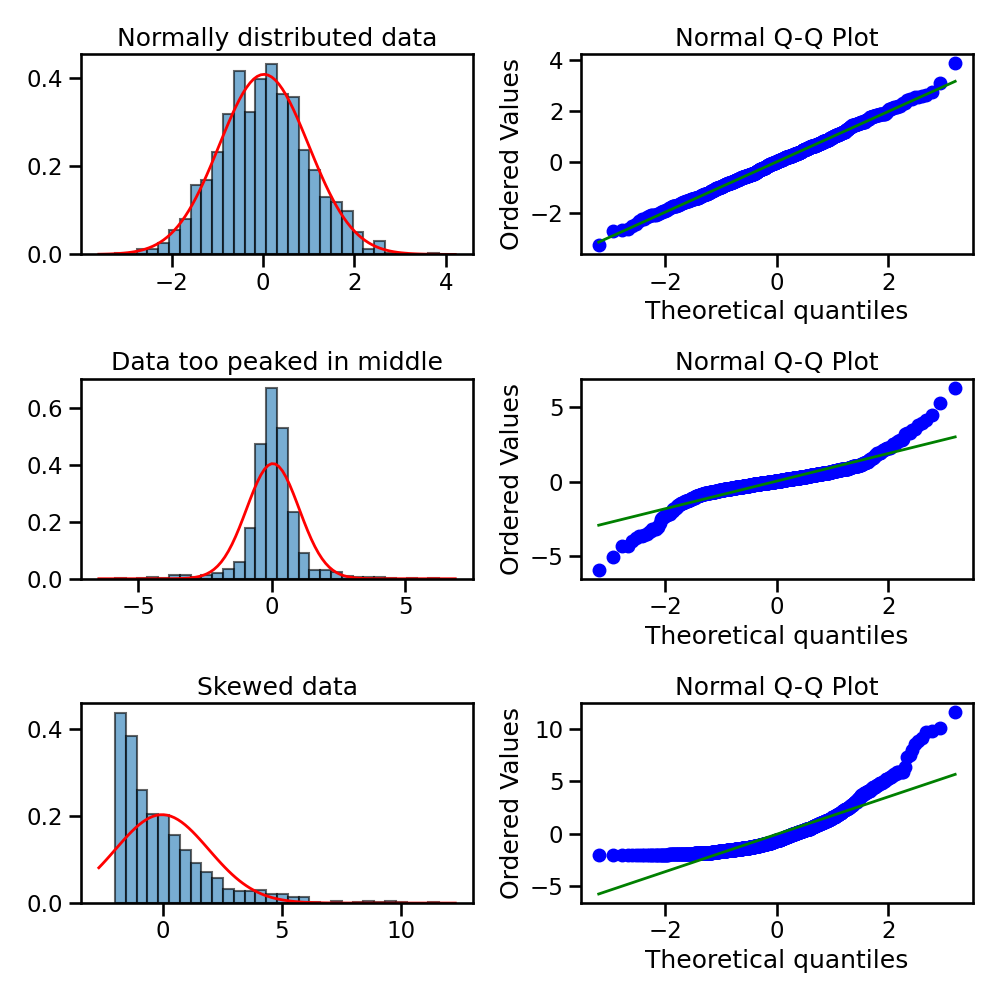
• In many data science projects, we still need to draw histogram plots or QQ (Quantile-Quantile) plot to check the normality.

QQ Plot vs Histogram

image

Special Case of \(\sigma_1\) and \(\sigma_2\) Unknown

Definition: Uses data from two samples with similar standard deviations (even though we don’t know their population std) to estimate a common standard deviation.

Formula (Pooled Standard Deviation): \[s^2_{\text{pooled}} = \frac{s^2_1 \times (n_1 - 1) + s^2_2 \times (n_2 - 1)}{n_1 + n_2 - 2}\] Degrees of freedom: \(df = n_1 + n_2 - 2\).

Benefits: Provides a better estimate for group standard deviation and a larger degrees of freedom for t-distribution.

Caution: Only pool when background research indicates nearly equal population standard deviations.

Data Science Example: Diamonds

• Weights of diamonds are measured in carats.

• 1 carat = 100 points, 0.99 carats = 99 points, etc.

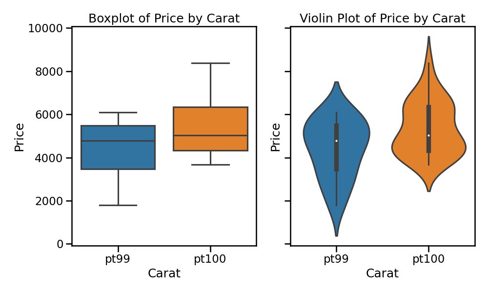
• The difference between the size of a 0.99 carat diamond and a 1 carat diamond is undetectable to the naked human eye, but does the price of a 1 carat diamond tend to be higher than the price of a 0.99 diamond?

• We are going to test to see if there is a difference between the average prices of 0.99 and 1 carat diamonds.

• In order to be able to compare equivalent units, we divide the prices of 0.99 carat diamonds by 99 and 1 carat diamonds by 100, and compare the average point prices.

image

Data

image

	0.99 carat	1 carat
	pt99	pt100
\(\bar{X}\)	44.50	53.43
\(s\)	13.32	12.22
\(n\)	23	30

Parameter and point estimate

• Parameter of interest: Average difference between the point prices of all 0.99 carat and 1 carat diamonds. \[\mu_{pt99} - \mu_{pt100}\]

  \(\:\)
  

• Point estimate: Average difference between the point prices of sampled 0.99 carat and 1 carat diamonds. \[\bar{X}_{pt99} - \bar{X}_{pt100}\]

Hypotheses

Which of the following is the correct set of hypotheses for testing if the average point price of 1 carat diamonds (\(_{pt100}\)) is higher than the average point price of 0.99 carat diamonds (\(_{pt99}\))?

1. \(H_0:\) \(\mu_{pt99} = \mu_{pt100}\)
   \(H_1:\) \(\mu_{pt99} \ne \mu_{pt100}\)

2. \(H_0:\) \(\mu_{pt99} = \mu_{pt100}\)
   \(H_1:\) \(\mu_{pt99} > \mu_{pt100}\)

3. \(H_0:\) \(\mu_{pt99} = \mu_{pt100}\)
   \(H_1:\) \(\mu_{pt99} < \mu_{pt100}\)

4. \(H_0:\) \(\bar{X}_{pt99} = \bar{X}_{pt100}\)
   \(H_1:\) \(\bar{X}_{pt99} < \bar{X}_{pt100}\)

Conditions

Which of the following does not need to be satisfied in order to conduct this hypothesis test using theoretical methods?

1. Point price of one 0.99 carat diamond in the sample should be independent of another, and the point price of one 1 carat diamond should independent of another as well.

2. Point prices of 0.99 carat and 1 carat diamonds in the sample should be independent.

3. Distributions of point prices of 0.99 and 1 carat diamonds should not be extremely skewed.

4. Both sample sizes should be at least 30.

Test statistic

Test statistic for inference on the difference of two small sample means The test statistic for inference on the difference of two means where \(\sigma_1\) and \(\sigma_2\) are unknown is the \(T\) statistic. \[t_{df} = \frac{\text{point estimate} - \text{null value}}{SE}\] where \[SE = \sqrt{ \frac{s_1^2}{n_1} + \frac{s_2^2}{n_2} } \qquad \text{ and } \qquad df = min(n_1 - 1, n_2 - 1)\]

Note: The calculation of the \(df\) is actually much more complicated. For simplicity we’ll use the above formula to estimate the true \(df\) when conducting the analysis by hand.

Test statistic (cont.)

	0.99 carat	1 carat
	pt99	pt100
\(\bar{x}\)	44.50	53.43
\(s\)	13.32	12.22
\(n\)	23	30

in context...

\[\begin{aligned} t &=& \frac{\text{point estimate} - \text{null value} }{SE} \\ &=& \frac{(44.50 - 53.43) - 0}{ \sqrt{\frac{13.32^2}{23} + \frac{12.22^2}{30} }} \\ &=& \frac{-8.93}{3.56} \\ &=& -2.507 \end{aligned}\]

Test statistic (cont.)

Which of the following is the correct \(df\) for this hypothesis test?

1. 22

2. 23

3. 30

4. 29

5. 52

\(\rightarrow df = min(n_{pt99} - 1, n_{pt100} - 1)\)
\(= min(23 - 1, 30 - 1)\)
\(= min(22,29) = 22\)

p-value

Which of the following is the correct p-value for this hypothesis test?

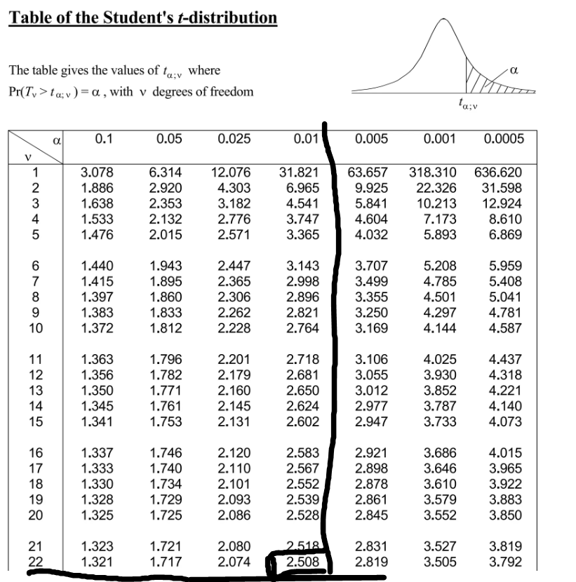
\[t = -2.507 \qquad df = 22\]

1. between 0.005 and 0.01

2. between 0.01 and 0.025

3. between 0.025 and 0.05

> stats.t.cdf(-2.507, 22)
[1] 0.010029001182850803

t-Table

image

Synthesis

What is the conclusion of the hypothesis test? How (if at all) would this conclusion change your behaviour if you went diamond shopping?

• p-value is small (< 5%) so reject \(H_0\). The data provide convincing evidence to suggest that the point price of 0.99 carat diamonds is lower than the point price of 1 carat diamonds.

• Maybe buy a 0.99 carat diamond? It looks like a 1 carat, but is significantly cheaper.

Equivalent confidence level

What is the equivalent confidence level for a one-sided hypothesis test at \(\alpha = 0.05\)?

1. 90%

2. 92.5%

3. 95%

4. 97.5%

image

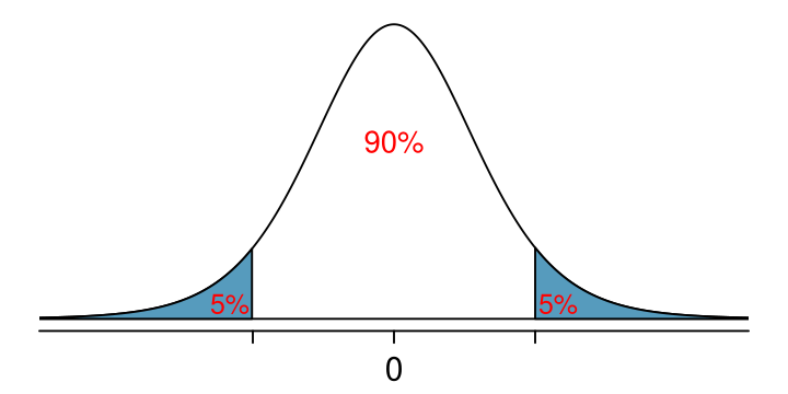
Correct Answer: 90%

Critical value

What is the appropriate \(t\) for a confidence interval for the average difference between the point prices of 0.99 and 1 carat diamonds?

1. 1.32

2. 1.72

3. 2.07

4. 2.82

> stats.t.ppf(0.95, 22)

[1] 1.717144

Confidence interval

Calculate the interval, and interpret it in context.

\[\text{point estimate} \pm ME\] \[\begin{aligned} (\bar{x}_{pt99} - \bar{x}_{pt100}) \pm t^\star_{df} \times SE &=& (44.50 - 53.43) \pm 1.72 \times 3.56 \\ &=& -8.93 \pm 6.12 \\ &=& (-15.05, -2.81) \end{aligned}\] We are 90% confident that the average point price of a 0.99 carat diamond is $15.05 to $2.81 lower than the average point price of a 1 carat diamond.

Recap: Inference using difference of two small sample means

• If \(\sigma_1\) or \(\sigma_2\) is unknown, difference between the sample means follow a \(t\)-distribution with \(SE = \sqrt{ \frac{s_1^2}{n_1} + \frac{s_2^2}{n_1} }\).

• Conditions:

  • independence within groups (often verified by a random sample, and if sampling without replacement, \(n <\) 10% of population) and between groups

  • no extreme skew in either group

• Hypothesis testing: \[t_{df} = \frac{\text{point estimate} - \text{null value}}{SE}\text{, where }df = min(n_1 - 1, n_2 - 1)\]

• Confidence interval: \[\text{point estimate} \pm t_{df}^\star \times SE\]

Two Population Means: Matched Samples

Matched Samples

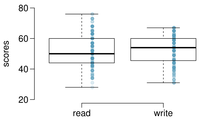
200 observations were randomly sampled from the High School and Beyond survey. The same students took a reading and writing test and their scores are shown below.

At a first glance, does there appear to be a difference between the average reading and writing test score?

image

Close look at the Data

The same students took a reading and writing test and their scores are shown below. Are the reading and writing scores of each student independent of each other?

	id	read	write
1	70	57	52
2	86	44	33
3	141	63	44
4	172	47	52
\(\vdots\)	\(\vdots\)	\(\vdots\)	\(\vdots\)
200	137	63	65

1. Yes

2. No

Analysing paired data

• When two sets of observations have this special correspondence (not independent), they are said to be paired/matched.

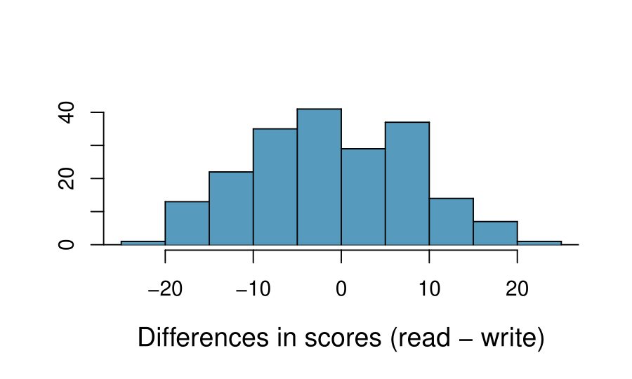
• To analyze paired data, it is often useful to look at the difference in outcomes of each pair of observations. \[\text{diff} = \text{read} - \text{write}\]

• It is important that we always subtract using a consistent order.

	id	read	write	diff
1	70	57	52	5
2	86	44	33	11
3	141	63	44	19
4	172	47	52	-5
\(\vdots\)	\(\vdots\)	\(\vdots\)	\(\vdots\)	\(\vdots\)
200	137	63	65	-2

image

Parameter and point estimate

• Parameter of interest: Average difference between the reading and writing scores of all high school students. \[\mu_{diff}\]

  \(\:\)
  

• Point estimate: Average difference between the reading and writing scores of sampled high school students. \[\bar{x}_{diff}\]

Setting the hypotheses

If in fact there was no difference between the scores on the reading and writing exams, what would you expect the average difference to be? \[\text{average diff} = 0\]

\(\:\)
What are the hypotheses for testing if there is a difference between the average reading and writing scores?

• There is no difference between the average reading and writing score. \[\mu_{diff} = 0\]

• There is a difference between the average reading and writing score. \[\mu_{diff} \ne 0\]

Nothing new here

• The analysis is no different than what we have done before.

• We have data from one sample: differences.

• We are testing to see if the average difference is different than 0.

Checking assumptions & conditions

Which of the following is true?

1. Since students are sampled randomly and are less than 10% of all high school students, we can assume that the difference between the reading and writing scores of one student in the sample is independent of another.

2. The distribution of differences is bimodal, therefore we cannot continue with the hypothesis test.

3. In order for differences to be random we should have sampled with replacement.

4. Since students are sampled randomly and are less than 10% all students, we can assume that the sampling distribution of the average difference will be nearly normal.

Calculating the test-statistic and the p-value

The observed average difference between the two scores is -0.545 points and the standard deviation of the difference is 8.887 points. Do these data provide convincing evidence of a difference between the average scores on the two exams? Use \(\alpha = 0.05\).

image

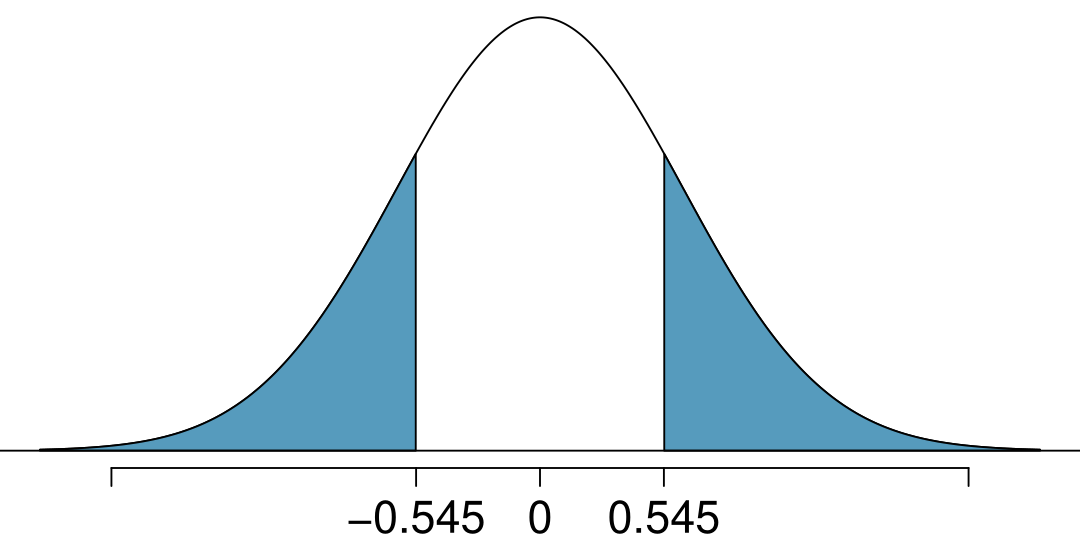
\[\begin{aligned} t &=& \frac{-0.545 - 0}{\frac{8.887}{\sqrt{200}}} \\ &=& \frac{-0.545}{0.628} = -0.87 \\ df &=& 200 - 1 = 199 \\ \text{p-value} &=& 0.1927 \times 2 = 0.3854 \end{aligned}\]

\(\:\)
Since p-value \(>\) 0.05, fail to reject, the data do not provide convincing evidence of a difference between the average reading and writing scores.

Interpretation of p-value

Which of the following is the correct interpretation of the p-value?

1. Probability that the average scores on the reading and writing exams are equal.

2. Probability that the average scores on the reading and writing exams are different.

3. Probability of obtaining a random sample of 200 students where the average difference between the reading and writing scores is at least 0.545 (in either direction), if in fact the true average difference between the scores is 0.

4. Probability of incorrectly rejecting the null hypothesis if in fact the null hypothesis is true.

HT \(\leftrightarrow\) CI

Suppose we were to construct a 95% confidence interval for the average difference between the reading and writing scores. Would you expect this interval to include 0?

1. yes

2. no

3. cannot tell from the information given

\[\begin{aligned} -0.545 \pm 1.97 \frac{8.887}{\sqrt{200}} &=& -0.545 \pm 1.97 \times 0.628 \\ &=& -0.545 \pm 1.24 \\ &=& (-1.785, 0.695) \end{aligned}\]

Correct Answer: (a)

Two Population Proportions

Digital Transformation in Banking

As banks undergo digital transformations, many are considering discontinuing physical branches in the next decade. How would this change impact your banking habits and preferences?

1. Significantly - I prefer in-person banking

2. Moderately - I use both online and in-person services

3. Minimally - I primarily use online services

4. Not at all - I exclusively bank online

Results from the UK

In the below there are the distributions of responses from Edinburgh University as well as from a group of students at York University:

	Edinburgh	York
Significantly	454	69
Moderately	124	30
Minimally	52	4
Not at all	50	2
Total	680	105

Parameter and point estimate

• Parameter of interest: Difference between the proportions of all York students and all Edinburgh who would who would say "significantly": \[ p_{YK} - p_{ED} \]

• Point estimate: Difference between the proportions of sampled York students and sampled Edinburgh who would say "significantly": \[ \hat{p}_{YK} - \hat{p}_{ED} \]

Inference for comparing proportions

• The details are the same as before...

• CI: \(point~estimate \pm margin~of~error\)

• HT: Use \(Z = \frac{point~estimate - null~value}{SE}\) to find appropriate p-value.

• We just need the appropriate standard error of the point estimate (\(SE_{ \hat{p}_{YK} - \hat{p}_{ED}}\)), which is the only new concept.

Standard error of the difference between two sample proportions \[SE_{(\hat{p}_1 - \hat{p}_2)} = \sqrt{ \frac{p_1(1-p_1)}{n_1} + \frac{p_2(1-p_2)}{n_2} }\]

Conditions for CI for difference of proportions

1. Independence within groups:

   • The ED group is sampled randomly and we’re assuming that the YK group represents a random sample as well.

   • 105 \(<\) 10% of all YK students and 680 \(<\) 10% of all ED.

   We can assume that the attitudes of YK students in the sample are independent of each other, and attitudes of ED students in the sample are independent of each other as well.

2. Independence between groups: The sampled YK students and the ED students are independent of each other.

3. Success-failure:
   At least 10 observed successes and 10 observed failures in the two groups.

Data

Construct a 95% confidence interval for the difference between the proportions of Duke students and Americans who would say "significantly": (\(p_{YK} - p_{ED}\)).

Data	YK	ED
Significantly	69	454
Not Significantly	36	226
Total	105	680
\(\hat{p}\)	0.657	0.668

\[\begin{aligned} && (\hat{p}_{YK} - \hat{p}_{ED}) \pm z^\star \times \sqrt{ \frac{ \hat{p}_{YK} (1 - \hat{p}_{YK})}{n_{YK} } + \frac{ \hat{p}_{ED} (1 - \hat{p}_{ED})}{n_{ED} } } \\ &=& (0.657 - 0.668) \pm 1.96 \times \sqrt{ \frac{0.657 \times 0.343}{105} + \frac{0.668 \times 0.332}{680} } \\ &=& -0.011 \pm 1.96 \times 0.0497 \\ &=& -0.011 \pm 0.097 \\ &=& (-0.108, 0.086) \end{aligned}\]

Hypothesis

Which of the following is the correct set of hypotheses for testing if the proportion of all YK students who would say "significantly" from the proportion of all ED who do?

1. \(H_0: p_{YK} = p_{ED}\)
   \(H_A: p_{YK} \ne p_{ED}\)

2. \(H_0: \hat{p}_{YK} = \hat{p}_{ED}\)
   \(H_A: \hat{p}_{YK} \ne \hat{p}_{ED}\)

3. \(H_0: p_{YK} - p_{ED} = 0\)
   \(H_A: p_{YK} - p_{ED} \ne 0\)

4. \(H_0: p_{YK} = p_{ED}\)
   \(H_A: p_{YK} < p_{ED}\)

Both (a) and (c) are correct.

Flashback to working with one proportion

• When constructing a confidence interval for a population proportion, we check if the observed number of successes and failures are at least 10. \[n\hat{p} \ge 10 \qquad \qquad n(1-\hat{p}) \ge 10\]

• When conducting a hypothesis test for a population proportion, we check if the expected number of successes and failures are at least 10. \[np_0 \ge 10 \qquad \qquad n(1-p_0) \ge 10\]

Pooled estimate of a proportion

• In the case of comparing two proportions where \(H_0: p_1 = p_2\), there isn’t a given null value we can use to calculated the expected number of successes and failures in each sample.

• Therefore, we need to first find a common (pooled) proportion for the two groups, and use that in our analysis.

• This simply means finding the proportion of total successes among the total number of observations.

\(\:\)
Pooled estimate of a proportion \[\hat{p} = \frac{\#~of~successes_1 + \#~of~successes_2}{n_1 + n_2}\]

Pooled Proportion

Calculate the estimated pooled proportion of YK and ED students who would say "Significantly". Which sample proportion (\(\hat{p}_{YK}\) or \(\hat{p}_{ED}\)) the pooled estimate is closer to? Why?

Data	YK	ED
A great deal	69	454
Not a great deal	36	226
Total	105	680
\(\hat{p}\)	0.657	0.668

\[\begin{aligned} \hat{p} &=& \frac{\#~of~successes_1 + \#~of~successes_2}{n_1 + n_2} \\ &=& \frac{69+454}{105+680} = \frac{523}{785} = 0.666 \end{aligned}\]

Test Statistic

Do these data suggest that the proportion of all YK students from the proportion of all ED who do? Calculate the test statistic, the p-value, and interpret your conclusion in context of the data.

Data	YK	ED
A great deal	69	454
Not a great deal	36	226
Total	105	680
\(\hat{p}\)	0.657	0.668

\[\begin{aligned} Z &=& \frac{(\hat{p}_{YK} - \hat{p}_{ED})}{\sqrt{ \frac{ \hat{p} (1 - \hat{p})}{n_{YK} } + \frac{ \hat{p} (1 - \hat{p})}{n_{ED} } }} \\ &=& \frac{(0.657 - 0.668)}{\sqrt{ \frac{0.666 \times 0.334}{105} + \frac{0.666 \times 0.334}{680} }} = \frac{-0.011}{0.0495} = -0.22 \\ p-value &=& 2 \times P(Z < -0.22) = 2 \times 0.41 = 0.82 \end{aligned}\]

Recap - comparing two proportions

• Population parameter: \((p_1 - p_2)\), point estimate: \((\hat{p}_1 - \hat{p}_2)\)

• Conditions:

  • independence within groups
    

    • random sample and 10% condition met for both groups

  • independence between groups

  • at least 10 successes and failures in each group
    

• \(SE_{(\hat{p}_1 - \hat{p}_2)} = \sqrt{ \frac{p_1(1-p_1)}{n_1} + \frac{p_2(1-p_2)}{n_2} }\)

  • for CI: use \(\hat{p}_1\) and \(\hat{p}_2\)

  • for HT:

  • when \(H_0: p_1 = p_2\): use \(\hat{p}_{pool} = \frac{\#~suc_1 + \#suc_2}{n_1 + n_2}\)

  • when \(H_0: p_1 - p_2 =\) (some value other than 0): use \(\hat{p}_1\) and \(\hat{p}_2\)
    

    • this is pretty rare

Reference - standard error calculations

           one sample                         two samples

---

mean \(SE = \frac{s}{\sqrt{n}}\) \(SE = \sqrt{ \frac{s_1^2}{n_1} + \frac{s_2^2}{n_2}}\)

proportion \(SE = \sqrt{ \frac{p(1-p)}{n} }\) \(SE = \sqrt{ \frac{p_1(1-p_1)}{n_1} + \frac{p_2(1-p_2)}{n_2} }\)

• When working with means, it’s very rare that \(\sigma\) is known, so we usually use \(s\).

• When working with proportions,

  • if doing a hypothesis test, \(p\) comes from the null hypothesis

  • if constructing a confidence interval, use \(\hat{p}\) instead