Statistics for Analytics

Session 7: Comparing Groups & Categorical Outcomes

Dr Zexun Chen

Zexun.Chen@ed.ac.uk

Today’s route

Match the method to the design, then explain the size and pattern of a group difference.

Teaching time: 110 minutes, plus a 10-minute break. The timed blocks include calculation, discussion and Wooclap debriefs.

• 000–005 min: Choose the outcome and study design
• 005–035 min: Independent means and the credit-limit calculation
• 035–055 min: Two proportions and the channel-claim activity
• 055–065 min: Break
• 065–095 min: Chi-square association, expected-count exercise and residuals
• 095–110 min: Goodness of fit, homogeneity distinction and categorical-test activity
• 110–120 min: Method choice, reporting and questions

Reference slides are available after the session takeaway and are not part of the core two-hour route.

Independent Means

A real credit-risk comparison

Credit limits differ between records with and without next-month default.

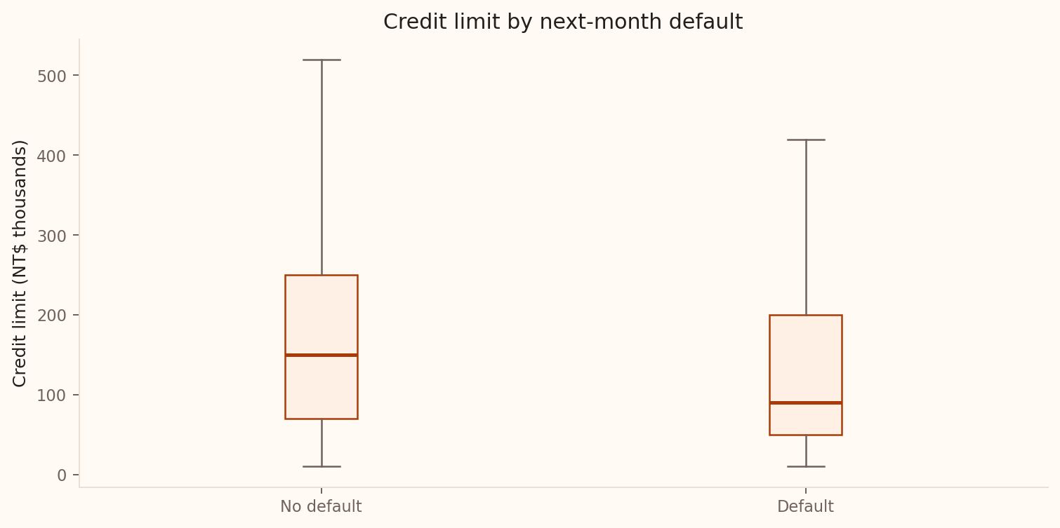
How large is the difference in mean credit limit between the two outcome groups?

Source: Yeh, UCI Default of Credit Card Clients. Groups are observational; outlier marks are hidden in the plot, not removed from calculations.

Parameter and estimate

\[\text{parameter: }\mu_1-\mu_2 \qquad \text{estimate: }\bar x_1-\bar x_2\]

The sign depends on the chosen order. Define Group 1 and Group 2 before calculating.

Welch two-sample test

For \(H_0:\mu_1-\mu_2=\Delta_0\):

\[SE=\sqrt{\frac{s_1^2}{n_1}+\frac{s_2^2}{n_2}},\]

\[t=\frac{(\bar x_1-\bar x_2)-\Delta_0}{SE}\]

Software calculates Welch–Satterthwaite degrees of freedom. Usually \(\Delta_0=0\).

The matching confidence interval is \((\bar x_1-\bar x_2)\pm t^*SE\).

Welch degrees of freedom are (s1^2/n1+s22/n2)^2 divided by [(s1^2/n1)2/(n1−1)+(s2^2/n2)2/(n2−1)]. Retain the software value when evaluating the t distribution. The test and interval both use the same SE and degrees of freedom.

Conditions

Independent groups

No unit in both

Independent within

Representative samples

Shape

Normal or large \(n\)

No extremes

At small \(n\)

Credit-limit summaries

Let Group 1 be no next-month default and Group 2 be default.

Outcome	\(n\)	Mean limit (NTD 000)	SD (NTD 000)
No default	23,364	178.10	131.63
Default	6,636	130.11	115.38

Difference estimate: \(178.10-130.11=47.99\) thousand NTD.

Source: UCI Default of Credit Card Clients; all 30,000 records.

Build the comparison before reading the result

For no-default versus default records, the mean limits are 178.10 and 130.11 thousand NTD.

The Welch standard error of their difference is 1.658 thousand NTD.

1. Estimate the difference and an approximate 95% interval using \(1.96\times SE\).
2. State which group’s mean is higher.
3. Explain whether the comparison establishes a lending-policy effect.

Allow 7 minutes within the independent-means block. Rounded calculation: difference 47.99, margin about 3.25, interval 44.74 to 51.24 thousand NTD. The large Welch degrees of freedom make 1.96 a useful approximation here. The next slide gives the model-based result from unrounded values. Observational groups do not identify what would happen if credit limits were changed.

Credit-limit comparison: the finding

\[H_0:\mu_1-\mu_2=0\qquad H_A:\mu_1-\mu_2\ne0\]

Welch’s test gives approximately

\[t=28.95,\qquad df\approx11{,}982.\]

\[p<.001.\]

Mean credit limit is 47.99 thousand NTD higher in the no-default group; the model-based 95% interval is 44.74 to 51.24 thousand NTD.

This compares observed groups. A lending intervention requires a different design.

These t results assume independent observations from the modelled populations. The published dataset does not document probability sampling from all bank customers. Its group difference is descriptive evidence; the model-based interval does not eliminate selection or confounding.

Two Proportions

Comparing rates

Group	Successes	Total	Sample proportion
Cellular	4,369	29,285	.1492
Telephone	390	2,906	.1342

Parameter: \(p_1-p_2\). Estimate: 1.50 percentage points, revisiting Week 1’s comparison.

Source: UCI Bank Marketing. “Success” is term-deposit subscription; this is an observational comparison.

Test of equal proportions

Under \(H_0:p_1=p_2\), pool the proportions:

\[\hat p_{pool}=\frac{x_1+x_2}{n_1+n_2}.\]

\[z=\frac{\hat p_1-\hat p_2} {\sqrt{\hat p_{pool}(1-\hat p_{pool})(1/n_1+1/n_2)}}.\]

Check independence within and between groups, and adequate expected successes and failures in each group.

Why pool only for the test?

Test

\(H_0\) says the proportions are equal, so one pooled estimate is coherent.

Interval

Does not assume equality, so keep separate estimates.

For the confidence interval, use

\[(\hat p_1-\hat p_2)\pm z^*\sqrt{\frac{\hat p_1(1-\hat p_1)}{n_1}+\frac{\hat p_2(1-\hat p_2)}{n_2}}.\]

Subscription-rate result

For 4,369/29,285 versus 390/2,906:

\[\hat p_{pool}=4759/32191=.1478,\qquad z=2.17,\qquad p=.030.\]

The estimated difference is 1.50 percentage points, with a 95% interval of 0.19 to 2.80 percentage points.

Next step: compare contact methods in a randomised campaign to assess their causal effect.

Values are calculated from unrounded rates. The 5% normal-approximation test provides evidence of an association under the independent-group model. Customer mix and campaign timing may explain it. The interval is a model-based comparison, not evidence that changing the channel would deliver the same increase.

What does the channel comparison establish?

The cellular minus telephone subscription difference is 1.50 percentage points, with a model-based 95% interval from 0.19 to 2.80. Which conclusion is supported?

1. Switching every client to cellular will cause a 1.50-point increase
2. The recorded groups differ; a randomised comparison could test a channel effect
3. Every cellular client is more likely to subscribe
4. The interval contains 95% of individual clients

Format: multiple choice, one answer; 90 seconds. Correct: option 2. Debrief: distinguish an estimated group difference from a causal treatment effect. Ask which customers could be included in a randomised comparison: those reachable by either method.

Categorical Association

Contact method and subscription

The real campaign data cross-classify last contact method and term-deposit outcome.

Contact	No	Yes	Total
Cellular	24,916	4,369	29,285
Telephone	2,516	390	2,906
Unknown	12,490	530	13,020
Total	39,922	5,289	45,211

Source: Moro, Rita & Cortez, UCI Bank Marketing. “Unknown” is an observed category, not missing-row deletion.

What independence predicts

Hypothesis	Claim about contact method and subscription
\(H_0\)	Independent
\(H_A\)	Associated

If \(H_0\) holds,

\[E_{ij}=\frac{(\text{row total})(\text{column total})}{n}\]

For Cellular × Yes:

\[E=29285\times5289/45211=3425.90.\]

Calculate one expected cell

Under independence, all contact groups share the overall subscription rate.

There are 13,020 unknown-method records, 5,289 subscriptions and 45,211 records in total.

1. Calculate the expected number of subscriptions in the unknown-method group.
2. Compare it with the observed 530.
3. Predict the sign of its Pearson residual and its contribution to \(\chi^2\).

Allow 6 minutes within the categorical-association block. Expected count = 13,020 × 5,289 / 45,211 = 1,523.14; observed is much lower. The Pearson residual is negative, about −25.45, while its squared contribution is positive, 647.56. The contribution table and heatmap follow. This task prepares students to explain which cells drive a significant global result.

Cell contributions

\[\chi^2=\sum\frac{(O-E)^2}{E}\]

Contact	No	Yes
Cellular	34.40	259.62
Telephone	0.98	7.37
Unknown	85.79	647.56

\[\chi^2=1035.71,\qquad df=(r-1)(c-1)=2.\]

Large values mean observed counts are far from independence.

Decision and interpretation

1035.71

Observed \(\chi^2\)

2

Degrees of freedom

\(<.001\)

p-value

At \(\alpha=.05\), the critical value is 5.991. Reject independence: contact method and subscription are associated.

The statistic is compared with the upper tail of a chi-square distribution with two degrees of freedom. For df=2, upper-tail critical values are 4.605 at .10, 5.991 at .05, 9.210 at .01, and 13.816 at .001. The reference distribution assumes independent units under the sampling model; the public campaign records do not establish representative sampling from all customers.

Which cells drive the result?

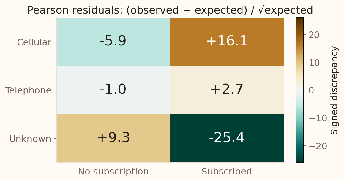
Next step: investigate the unknown-method group and differences in customer mix before changing campaign policy.

UCI Bank Marketing. Squaring and summing these Pearson residuals gives the chi-square statistic.

Unknown method has 530 subscriptions versus 1,523.14 expected under independence. Its Yes cell contributes 647.56, the largest contribution. Cellular has 4,369 subscriptions versus 3,425.90 expected. The signs of the residuals show direction; the squared contributions show how much each cell adds to the test statistic.

Conditions

Counts

Not percentages

Independent

One cell per unit

Expected

All at least 5 here

Representative

Valid sampling

Each unit contributes to exactly one cell and units should be independent. All expected counts at least five is a simple sufficient classroom check. Sparse tables may need an exact test or simulation; combine categories only when the substantive meaning supports it. Representative selection is needed to generalise to a specified population.

Strength, not only significance

For an \(r\times c\) table, Cramér’s V is

\[V=\sqrt{\frac{\chi^2}{n\min(r-1,c-1)}}.\]

For these data,

\[V=\sqrt{1035.71/(45211\times1)}=.151.\]

This quantifies association strength on a 0–1 scale.

Benchmarks & Method Choice

One variable, specified distribution

Goodness of fit compares observed category counts with proportions specified by \(H_0\).

\[H_0:p_1=p_{1,0},\ldots,p_k=p_{k,0}\]

\[E_i=np_{i,0},\qquad df=k-1-m,\]

where \(m\) parameters were estimated from the data.

Account preferences: a planning check

An illustrative survey of 300 customers is compared with a prespecified account-preference mix.

Account type	Observed	Planned share	Expected
Savings	140	50%	150
Current	90	30%	90
Investment	70	20%	60

\[\chi^2=\frac{(140-150)^2}{150}+0+\frac{(70-60)^2}{60}=2.33.\]

With \(df=2\), \(p=.311\): insufficient evidence that preferences differ from the plan.

Illustrative example. The benchmark must be set before inspecting the survey results.

The expected counts are 300 times the planned proportions. All are at least five. Failing to reject the null does not prove that the underlying shares equal the plan exactly.

Choose the categorical test

Question	Test	Example
Are two variables related in one population?	Association	Contact method and subscription
Does one distribution match a benchmark?	Goodness of fit	Account preferences versus the plan
Is a distribution shared across populations?	Homogeneity	Account preferences in three regions

All compare observed counts with expected counts under the null.

Choose the categorical test

Match these questions: contact method and subscription in one customer sample; account preferences against a 50/30/20 benchmark; account preferences in separate samples from three regions.

Format: matching; two minutes. Answers in order: association or independence, goodness of fit, homogeneity. Debrief: the collection design and null hypothesis distinguish the tests, even when two use the same contingency-table calculation.

A compact decision map

Outcome	Design	Procedure
Numerical	Two independent groups	Welch two-sample t
Numerical	Paired observations	One-sample t on differences
Binary	Two independent groups	Two-proportion z
Categorical	Two variables in one sample	Chi-square association
Categorical	One variable versus specified shares	Chi-square goodness of fit

Ask about outcome type and study design before choosing a formula.

Session 7 takeaway

• Use Welch inference for independent means and preserve the group order.
• Use the null model to choose the test standard error.
• Chi-square tests compare observed counts with expected counts.
• Explain the pattern and effect size as well as the global p-value.

Next: compare several means and fit a line to a numerical outcome.

Reference

When both population SDs are known

\[SE=\sqrt{\frac{\sigma_1^2}{n_1}+\frac{\sigma_2^2}{n_2}},\qquad z=\frac{(\bar x_1-\bar x_2)-\Delta_0}{SE}.\]

Illustrative loan processing times:

Process	\(n\)	Mean (days)	Known SD (days)
A	50	7.0	2.0
B	60	6.5	2.5

Difference \(=.5\) day; \(SE=.429\); 95% interval \(=(-.34,1.34)\) days.

The population SDs are assumed known for these illustrative processes. The interval includes zero. If those SDs are estimated from the samples, use the appropriate t procedure instead.

Why not pool automatically?

The pooled t-test assumes \(\sigma_1^2=\sigma_2^2\).

Situation	Preferred approach
Variances may differ	Welch t
Strong equal-variance justification	Pooled t
Severe skew or extremes	Transform, robust, or randomisation method

With justified equal population variances, pooled variance is sp^{2=[(n1−1)s1}2+(n2−1)s2^2]/(n1+n2−2), pooled SE=sp sqrt(1/n1+1/n2), and df=n1+n2−2. Welch is the default here because it does not require equality. Assess skew and extreme values in plots; a preliminary variance test is not a substitute for choosing an appropriate mean-comparison method.

Relative measures

Measure	Estimate	Interpretation
Rate difference	\(\hat p_1-\hat p_2=.0150\)	+1.50 percentage points
Rate ratio	\(\hat p_1/\hat p_2=1.11\)	About 11% higher rate
Odds ratio	\(\frac{\hat p_1/(1-\hat p_1)}{\hat p_2/(1-\hat p_2)}=1.13\)	About 13% higher odds

The clearest measure depends on the decision context.

Expected counts

Contact	No	Yes	Total
Cellular	25,859.10	3,425.90	29,285
Telephone	2,566.04	339.96	2,906
Unknown	11,496.86	1,523.14	13,020
Total	39,922	5,289	45,211

Expected counts preserve the observed margins.

Homogeneity: compare category distributions

Question: Do account preferences have the same distribution across three regions?

Take a separate random sample of customers in each region and record Savings, Current, or Investment.

\[H_0:\text{The three regions have the same preference distribution.}\]

Use the same expected-count and chi-square formulas as an association test; here \(df=(3-1)(3-1)=4\).

The distinction is in the design: independence cross-classifies two variables from one sample; homogeneity compares a categorical outcome across separately sampled populations or assigned groups. Both use the same contingency-table calculation and need independent observations and adequate expected counts.

Checking a continuous distribution

A chi-square goodness-of-fit test can compare binned numerical data with a proposed distribution.

Step	Example: a normal model for settlement errors
Define bins	Cover the full range, including both tails
Find probabilities	\(p_i=F(b_i)-F(a_i)\) for each bin
Find expected counts	\(E_i=np_i\); keep expected counts adequate
Calculate	\(\chi^2=\sum(O_i-E_i)^2/E_i\)

Adjust degrees of freedom for fitted parameters: \(df=k-1-m\).

With six categories and mean and SD estimated as part of the grouped normal-fit procedure, the usual chi-square reference has df=6−1−2=3. With a fully specified distribution it has df=5. Use an estimation method and calibration appropriate to the binned test. The result depends on binning, so also inspect a histogram and Q–Q plot. A goodness-of-fit test does not require unordered categories; numerical intervals are valid categories.