Travel Preferences Survey
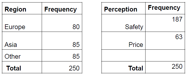
A survey has been conducted among subscribers to the newsletter by Visit Scotland about their travel plans next summer.
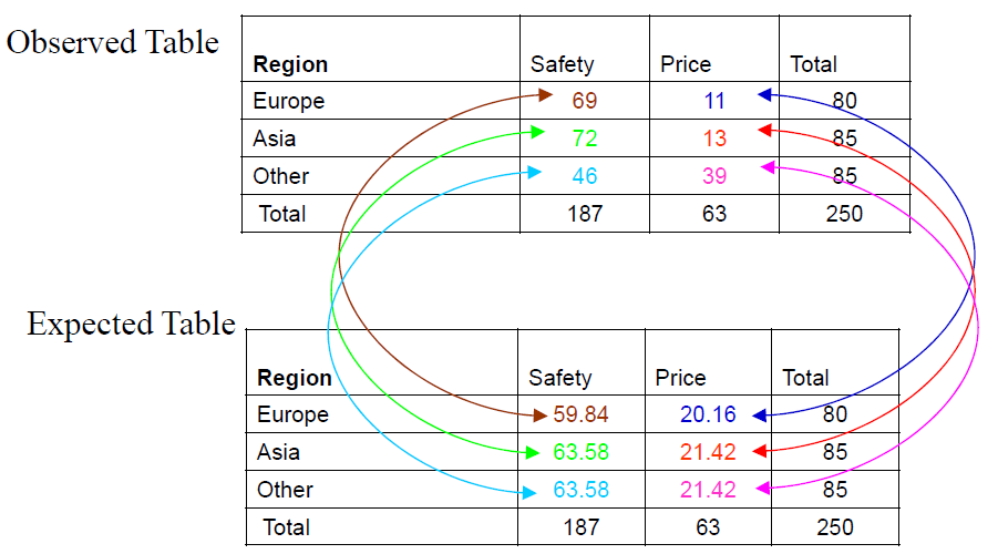
Is there a relationship between Region and Perceived Importance of Safety vs Price (Perception)?
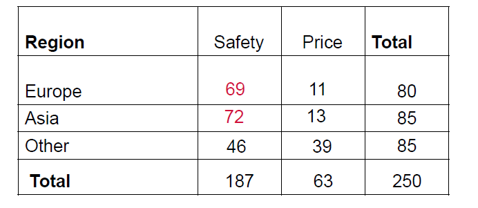
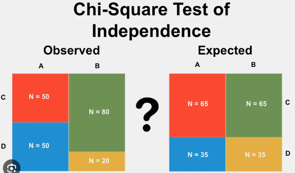
Contingency Table
If the Totals and just two numbers in the middle are known, one can fill in the rest of the table
This table has 2 degrees of freedom (df) \[\text{df = (\# rows - 1)} \times \text{(\# columns - 1)}\]
Hypotheses
If we are interested in proving that there is a relationship, this should be the alternative hypothesis.
Statistical Independence
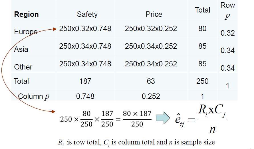
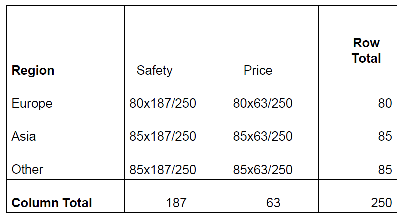
What use is Expected Value
Can Compare the Expected Value \(e_{ij}\) with Observed Value \(o_{ij}\)
If \(e_{ij}\) is close to \(o_{ij}\), then \(H_0\) is likely to be true.
If \(e_{ij}\) is NOT close to \(o_{ij}\), then \(H_1\) is likely to be true.
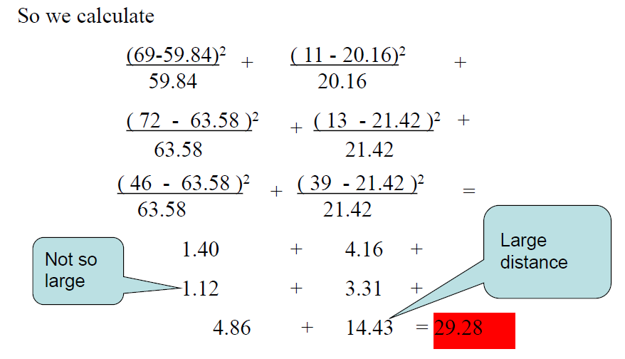
How Close? What Measure?
Pearson Chi Square Statistic - \(\chi^2\) \[\chi^2 = \sum_{i=1}^{r}\sum_{j=1}^{c} \frac{(o_{ij} - \hat{e}_{ij})^2}{\hat{e}_{ij}}\]
Why Square?
Remove Sign: Squaring ensures all differences are positive, focusing on the magnitude of deviation.
Emphasise Larger Discrepancies: Squaring gives more weight to larger differences, which are more indicative of a true discrepancy from the null hypothesis.
Distribution: The sum of squared standardised differences follows a Chi-Square distribution if the null hypothesis is true, allowing for theoretical comparison and p-value calculation.
Variances and Standard Deviations: Squaring differences relate to the concept of variance, which measures dispersion, making the Chi-Square test a form of variance measure.
The Chi-Square statistic is used to determine the probability of observing a test statistic as extreme as the one calculated, under the assumption of the null hypothesis.
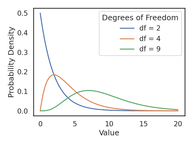
Chi-Square Distribution
In order to determine if \(\chi^2\) statistic we calculated is considered as "unusually" high or not we need to first describe its distribution
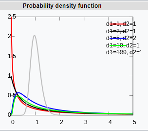
The chi-square distribution has just one parameter called degrees of freedom (df), which influences the shape, centre, and spread of the distribution.
The chi-squared distribution is the sum of squared standardised normal random variables such as \((Z_1)^2 + (Z_2)^2 + (Z_3)^2\) and so on.
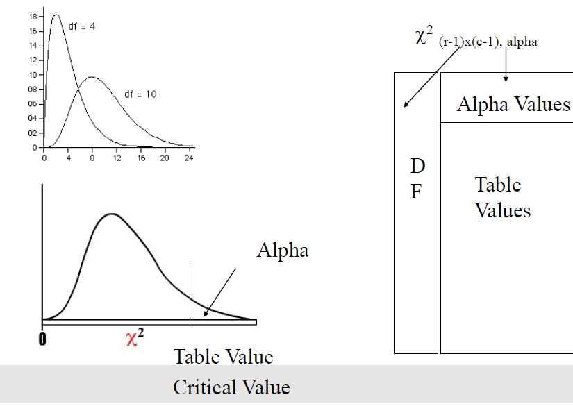
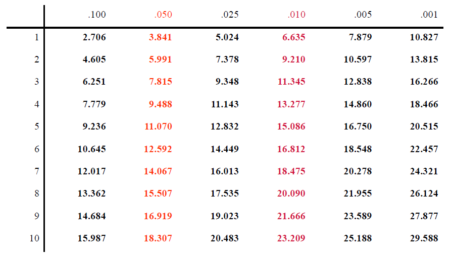
Chi-Square Distribution and Table
Chi-Square Table & Software
> scipy.stats.chi2.ppf(1-0.05, 2) # critical value, 1-alpha
[1] 5.991464547107979
> scipy.stats.chi2.isf(0.05, 2) # critical value, alpha
[1] 5.991464547107983
> scipy.stats.chi2.sf(29.28, 2) # p-value
[2] 4.3845879395753135e-07
> scipy.stats.chi2.cdf(29.28, 2) # If we need p-value, 1- cdf
[3] 0.9999995615412061
Steps: Chi-Square Test for Association
Formulate \(H_0\) and \(H_1\).
Specify the level of significance and test statistic.
Calculate Test Statistic using Observed Table:
Calculate Expected Table using \(\hat{e}_{ij} = \frac{R_i \times C_j}{n}\)
Calculate Pearson Chi Squared Statistic \(\chi^2 = \sum_{i=1}^{r} \sum_{j=1}^{c} \frac{(o_{ij} - \hat{e}_{ij})^2}{\hat{e}_{ij}}\)
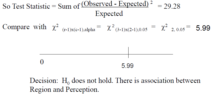
Critical region and critical value \(\chi^2\): (r-1)(c-1), \(\alpha\).
Decide on Hypotheses and Interpret Decision.
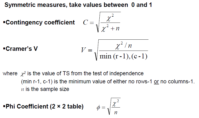
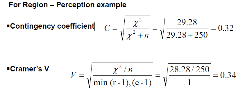
Measures of Association Nominal Data
Measures of Association Nominal Data
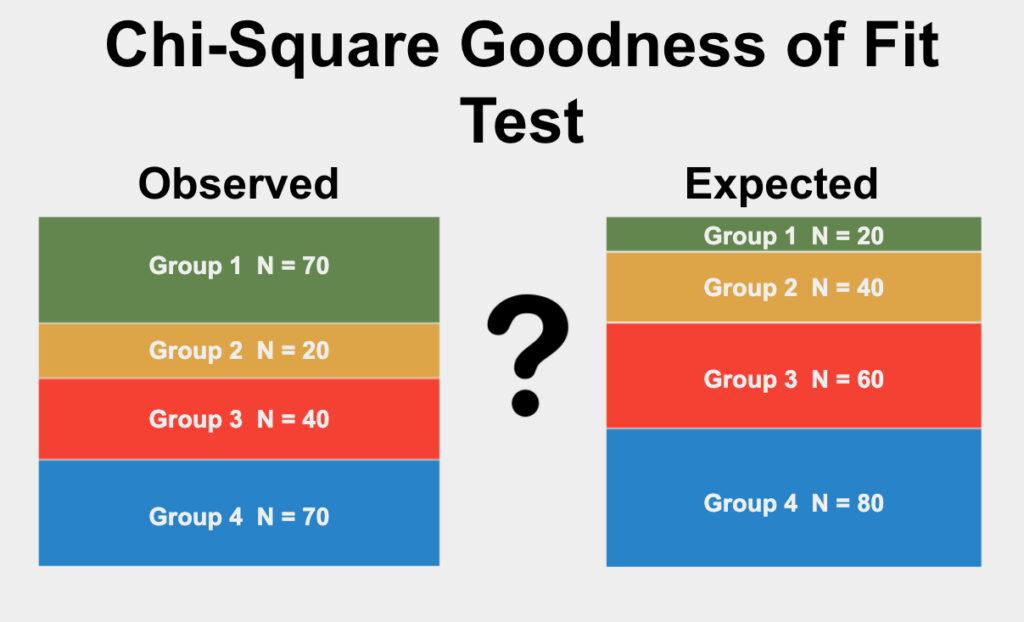
Account Type Preferences Among Bank Customers
Background: The bank offers three types of accounts and has expectations for the distribution of customer preferences.
Objective: To determine if the observed preferences fit the expected distribution using a Chi-square test of goodness of fit.
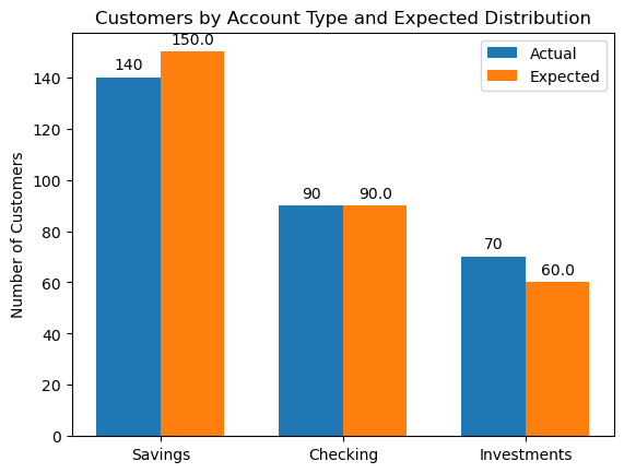
Data Collection: A survey of 300 customers yielded the following preferences:
Expected Distribution:
Savings: 50%
Checking: 30%
Investments: 20%
Hypotheses: \[H_0: \text{The distribution of preferences matches the expected.}\] \[H_1: \text{The distribution of preferences does not match the expected.}\]
Solution
Expected Frequencies:
Savings: \(E_{\text{Savings}} = 300 \times 0.50 = 150\)
Checking: \(E_{\text{Checking}} = 300 \times 0.30 = 90\)
Investments: \(E_{\text{Investments}} = 300 \times 0.20 = 60\)
Chi-Square Statistic Calculation: \[\chi^2 = \frac{(140 - 150)^2}{150} + \frac{(90 - 90)^2}{90} + \frac{(70 - 60)^2}{60} = 2.33\]
Degrees of Freedom: \[df = 3 - 1 = 2\]
Critical Value: Find from Chi-square table or statistical software for \(df = 2\) at \(\alpha = 0.05\) (\(\chi^2_{2, 0.05} = 5.99\)).
Decision: Compare the calculated \(\chi^2\) to the critical value to decide on \(H_0\).
- Insufficient evidence to reject \(H_0\) (2.33 < 5.99), match the expectation.
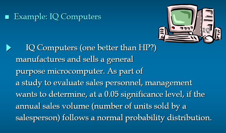
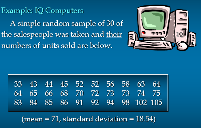
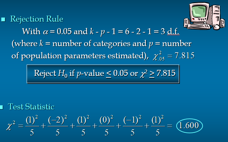
IQ-Computer: Normal Distribution Goodness of Fit Test
IQ-Computer: Normal Distribution Goodness of Fit Test
Hypothesis
\(H_0\): The population of number of units sold has a normal distribution with mean 71 and standard deviation 18.54.
\(H_1\): The population of number of units sold does NOT have a normal distribution with mean 71 and standard deviation 18.54.
Interval Definition
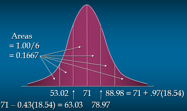
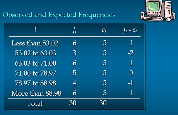
To satisfy the requirement of an expected frequency of at least 5 in each interval we will divide the normal distribution into 30/5 = 6 equal probability intervals.
Observed and Expected Frequencies
ANOVA
ANOVA (Analysis of Variance ) is used to assess whether the mean of the outcome variable is different for different levels of a categorical variable.
\(H_0:\) The mean outcome is the same across all categories, \[\mu_1 = \mu_2 = \cdots = \mu_k,\] where \(\mu_i\) represents the mean of the outcome for observations in category \(i\).
\(H_1:\) At least one mean is different than others.
Conditions
The observations should be independent within and between groups
If the data are a simple random sample from less than 10% of the population, this condition is satisfied.
Carefully consider whether the data may be independent (e.g. no pairing).
Always important, but sometimes difficult to check.
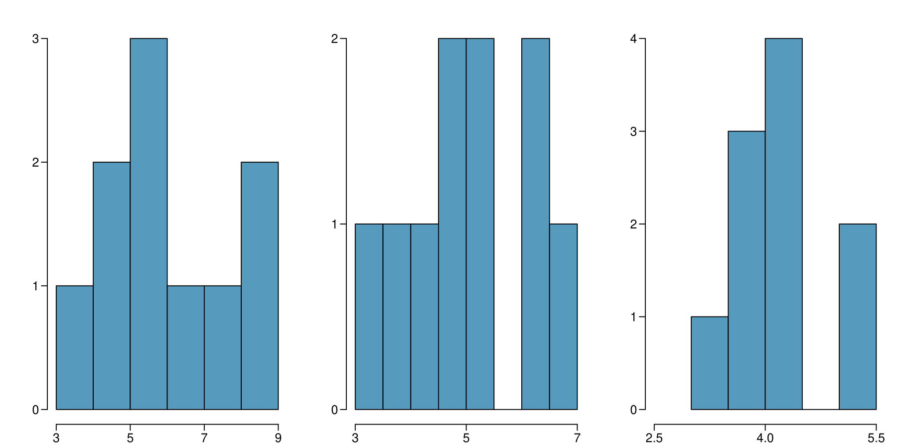
The observations within each group should be nearly normal.
- Especially important when the sample sizes are small.
The variability across the groups should be about equal.
- Especially important when the sample sizes differ between groups.
\(z\)/\(t\) test vs. ANOVA - Purpose
\[z/t\text{ test}\] Compare means from two groups to see whether they are so far apart that the observed difference cannot reasonably be attributed to sampling variability. \[H_0: \mu_1 = \mu_2\]
\[ANOVA\] Compare the means from two or more groups to see whether they are so far apart that the observed differences cannot all reasonably be attributed to sampling variability. \[H_0: \mu_1 = \mu_2 = \cdots = \mu_k\]
\(z\)/\(t\) test vs. ANOVA - Method
\[z/t\text{ test}\] Compute a test statistic (a ratio). \[z / t = \frac{(\bar{x}_1 - \bar{x}_2) - (\mu_1 - \mu_2)}{SE_{\bar{x}_1 - \bar{x}_2}}\]
\[ANOVA\] Compute a test statistic (a ratio). \[F = \frac{\text{variability bet. groups}}{\text{variability w/in groups}}\]
Large test statistics lead to small p-values.
If the p-value is small enough \(H_0\) is rejected, we conclude that the population means are not equal.
\(z\)/\(t\) test vs. ANOVA
With only two groups t-test and ANOVA are equivalent, but only if we use a pooled standard variance in the denominator of the test statistic.
With more than two groups, ANOVA compares the sample means to an overall grand mean.
Example Data
| bottom |
10 |
6.04 |
1.58 |
| middepth |
10 |
5.05 |
1.10 |
| surface |
10 |
4.20 |
0.66 |
| overall |
30 |
5.1 0 |
1.37 |
Hypotheses
What are the correct hypotheses for testing for a difference between the means among these groups?
\(H_0: \mu_B = \mu_M = \mu_S\)
\(H_1: \mu_B \ne \mu_M \ne \mu_S\)
\(H_0: \mu_B \ne \mu_ M \ne \mu_S\)
\(H_1: \mu_B = \mu_M = \mu_S\)
\(H_0: \mu_B = \mu_M = \mu_S\)
\(H_1:\) At least one mean is different.
\(H_0: \mu_B = \mu_M = \mu_S = 0\)
\(H_1:\) At least one mean is different.
\(H_0: \mu_B = \mu_M = \mu_S\)
\(H_1: \mu_B > \mu_M > \mu_S\)
Test statistic
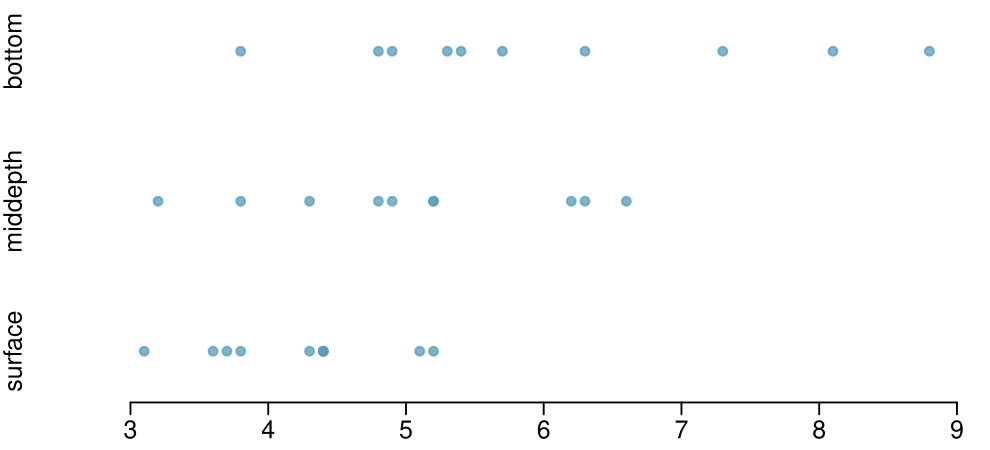
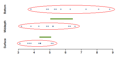
Does there appear to be a lot of variability within groups? How about between groups?
Total Variability = sum up (each observation - grand mean)\(^2\)
Between group variability = sum up (each group’s mean - grand mean)\(^2\)
Within group variability = Total variability - between group variability
\[F = \frac{\text{variability bet. groups}}{\text{variability w/in groups}}\]
\(F\) distribution and p-value
\[F = \frac{\text{variability bet. groups}}{\text{variability w/in groups}}\]
In order to be able to reject \(H_0\), we need a small p-value, which requires a large F statistic.
In order to obtain a large F statistic, variability between sample means needs to be greater than variability within sample means.
Degrees of freedom associated with ANOVA
| (Group) |
depth |
2 |
16.96 |
8.48 |
6.13 |
0.0063 |
| (Error) |
Residuals |
27 |
37.33 |
1.38 |
|
|
|
Total |
29 |
54.29 |
|
|
|
Degrees of freedom associated with ANOVA
groups: \(df_G = k - 1\), where \(k\) is the number of groups
total: \(df_T = n - 1\), where \(n\) is the total sample size
error: \(df_E = df_T - df_G\)
Sum of squares between groups, SSG
| (Group) |
depth |
2 |
16.96 |
8.48 |
6.13 |
0.0063 |
| (Error) |
Residuals |
27 |
37.33 |
1.38 |
|
|
|
Total |
29 |
54.29 |
|
|
|
Sum of squares between groups, SSG Measures the variability between groups \[SSG = \sum_{i = 1}^{k} n_i (\bar{x}_i - \bar{x})^2\] where \(n_i\) is each group size, \(\bar{x}_i\) is the average for each group, \(\bar{x}\) is the overall (grand) mean.
| bottom |
10 |
6.04 |
| middepth |
10 |
5.05 |
| surface |
10 |
4.2 |
| overall |
30 |
5.1 |
\[\begin{aligned}
SSG &=& \left( 10 \times (6.04 - 5.1)^2 \right) \\
&+& \left( 10 \times (5.05 - 5.1)^2 \right) \\
&+& \left( 10 \times (4.2 - 5.1)^2 \right) \\
&=& 16.96 \\
\end{aligned}\]
Sum of squares total, SST
| (Group) |
depth |
2 |
16.96 |
8.48 |
6.13 |
0.0063 |
| (Error) |
Residuals |
27 |
37.33 |
1.38 |
|
|
|
Total |
29 |
54.29 |
|
|
|
Sum of squares total, SST Measures the variability in total \[SST = \sum_{i = 1}^{n} (x_i - \bar{x})^2\] where \(x_i\) represent each observation in the dataset.
\[\begin{aligned}
SST &=& (3.8 - 5.1)^2 + (4.8 - 5.1)^2 + (4.9 - 5.1)^2 + \cdots + (5.2 - 5.1)^2 \\
&=& (-1.3)^2 + (-0.3)^2 + (-0.2)^2 + \cdots + (0.1)^2 \\
&=& 1.69 + 0.09 + 0.04 + \cdots + 0.01 \\
&=& 54.29
\end{aligned}\]
Sum of squares error, SSE
| (Group) |
depth |
2 |
16.96 |
8.48 |
6.13 |
0.0063 |
| (Error) |
Residuals |
27 |
37.33 |
1.38 |
|
|
|
Total |
29 |
54.29 |
|
|
|
Sum of squares error, SSE Measures the variability within groups: \[SSE = SST - SSG\]
\[SSE = 54.29 - 16.96 = 37.33\]
Mean square error
| (Group) |
depth |
2 |
16.96 |
8.48 |
6.13 |
0.0063 |
| (Error) |
Residuals |
27 |
37.33 |
1.38 |
|
|
|
Total |
29 |
54.29 |
|
|
|
Mean square error Mean square error is calculated as sum of squares divided by the degrees of freedom.
\[\begin{aligned}
MSG &=& 16.96 / 2 = 8.48 \\
MSE &=& 37.33 / 27 = 1.38
\end{aligned}\]
Test statistic, F value
| (Group) |
depth |
2 |
16.96 |
8.48 |
6.14 |
0.0063 |
| (Error) |
Residuals |
27 |
37.33 |
1.38 |
|
|
|
Total |
29 |
54.29 |
|
|
|
Test statistic, F value As we discussed before, the F statistic is the ratio of the between group and within group variability. \[F = \frac{MSG}{MSE}\]
\[F = \frac{8.48}{1.38} = 6.14\]
p-value
| (Group) |
depth |
2 |
16.96 |
8.48 |
6.14 |
0.0063 |
| (Error) |
Residuals |
27 |
37.33 |
1.38 |
|
|
|
Total |
29 |
54.29 |
|
|
|
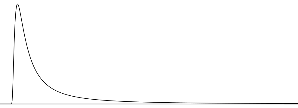
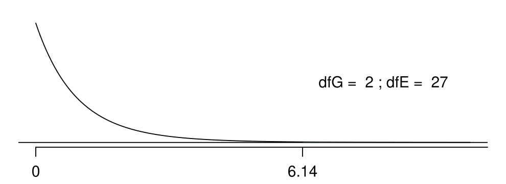
p-value p-value is the probability of at least as large a ratio between the “between group" and”within group" variability, if in fact the means of all groups are equal. It’s calculated as the area under the F curve, with degrees of freedom \(df_G\) and \(df_E\), above the observed F statistic.
![]()
image
Conclusion - in context
What is the conclusion of the hypothesis test?
\(\:\)
The data provide convincing evidence that the average mean
is different for all groups.
on the surface is lower than the other levels.
is different for at least one group.
is the same for all groups.
Conclusion
If p-value is small (less than \(\alpha\)), reject \(H_0\). The data provide convincing evidence that at least one mean is different from (but we can’t tell which one).
If p-value is large, fail to reject \(H_0\). The data do not provide convincing evidence that at least one pair of means are different from each other, the observed differences in sample means are attributable to sampling variability (or chance).
(1) independence
Does this condition appear to be satisfied?
(2) approximately normal
Does this condition appear to be satisfied?
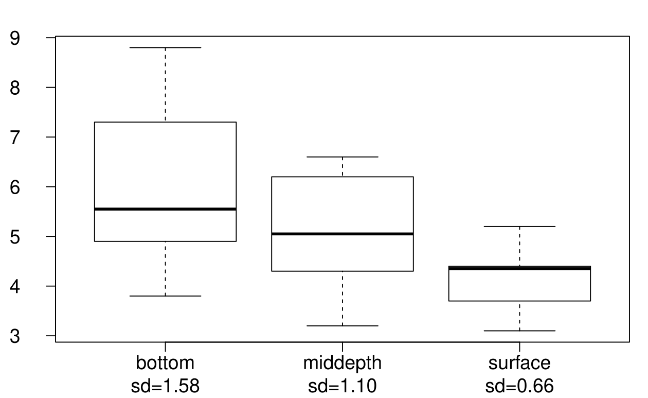
(3) constant variance
Does this condition appear to be satisfied?
Which means differ?
Based on the box plots below, which means would you expect to be significantly different?
bottom & surface
bottom & mid-depth
mid-depth & surface
bottom & mid-depth; mid-depth & surface
bottom & mid-depth; bottom & surface; mid-depth & surface
Which means differ? (cont.)
If the ANOVA assumption of equal variability across groups is satisfied, we can use the data from all groups to estimate variability:
Estimate any within-group standard deviation with \(\sqrt{MSE}\), which is \(s_{pooled}\)
Use the error degrees of freedom, \(n - k\), for \(t\)-distributions
Difference in two means: after ANOVA \[SE = \sqrt{ \frac{\sigma_1^2}{n_1} + \frac{\sigma_2^2}{n_2} } \approx \sqrt{ \frac{MSE}{n_1} + \frac{MSE}{n_2} }\]
Is there a difference between the mean at the bottom and at mid-depth?
Is there a difference between the mean at the bottom and at mid-depth?
| bottom |
10 |
6.04 |
1.58 |
| middepth |
10 |
5.05 |
1.10 |
| surface |
10 |
4.2 |
0.66 |
| overall |
30 |
5.1 |
1.37 |
| depth |
2 |
16.96 |
8.48 |
6.13 |
0.0063 |
| Residuals |
27 |
37.33 |
1.38 |
|
|
| Total |
29 |
54.29 |
|
|
|
$$
\[\begin{aligned}
T_{df_E} &=& \frac{(\bar{x}_{bottom} - \bar{x}_{middepth})}{\sqrt{ \frac{MSE}{n_{bottom}} + \frac{MSE}{n_{middepth}} }} \\
T_{27} &=& \frac{( 6.04 - 5.05 )}{\sqrt{ \frac{1.38}{10} + \frac{1.38}{10} }} = \frac{0.99}{0.53} =1.87 \\
0.05 &<& p-value < 0.10 \qquad \text{(two-sided)} \\
% \alpha^\star &=& 0.05 / 3 = 0.0167
\end{aligned}\]
$$