Statistics for Analytics

Session 8: ANOVA & Regression

Dr Zexun Chen

Zexun.Chen@ed.ac.uk

Today’s route

Explain variation with groups and fitted lines, then interpret an adjusted model.

Teaching time: 110 minutes, plus a 10-minute break. The timed blocks include calculation, discussion and Wooclap debriefs.

• 000–005 min: From two groups to several
• 005–035 min: ANOVA, assumptions, follow-up comparisons and activity
• 035–055 min: Correlation, its Wooclap check, fitted lines, least squares and slope activity
• 055–065 min: Break
• 065–085 min: Prediction and explained variation
• 085–100 min: Slope inference, model conditions and residual check
• 100–115 min: First multiple regression: indicators and adjusted interpretation
• 115–120 min: Synthesis and questions

Reference slides are available after the session takeaway and are not part of the core two-hour route.

Comparing Several Means

Why not many t-tests?

With \(k\) groups there are \(k(k-1)/2\) pairwise comparisons.

For 5 groups, that is 10 tests. At \(.05\) per test, the chance of at least one false positive can be much greater than 5%.

ANOVA starts with one global question.

The ANOVA hypotheses

\[H_0:\mu_1=\mu_2=\cdots=\mu_k\]

\[H_A:\text{not all population means are equal}\]

Rejecting \(H_0\) establishes that at least one mean differs. Follow-up comparisons identify which ones.

Real credit-limit groups

Question: Do mean credit limits differ across three recorded education groups?

Education	\(n\)	Mean (NTD 000)	SD (NTD 000)
Graduate school	10,585	212.96	135.47
University	14,030	147.06	120.67
High school	4,917	126.55	113.98

Grand mean across these 29,532 records: 167.27 thousand NTD.

Source: Yeh, UCI Default of Credit Card Clients. Records with “other/unknown” education codes are excluded from this three-group example.

Signal versus noise

\[F=\frac{\text{variation between group means}} {\text{variation within groups}}=\frac{MSG}{MSE}\]

Large \(F\) means group separation is large relative to background variation.

Partitioning variation

\[SST=SSG+SSE\]

Source	Variation	Degrees of freedom
Groups, \(SSG\)	Between group means	\(k-1\)
Error, \(SSE\)	Within groups	\(N-k\)
Total, \(SST\)	Around the grand mean	\(N-1\)

The degrees of freedom also partition: \((k-1)+(N-k)=N-1\).

ANOVA result

Source	SS (thousand NTD)\(^2\)	df	MS	F
Groups	35,975,139	2	17,987,570	1,148.68
Error	462,405,654	29,529	15,659
Total	498,380,793	29,531

\(p<.001\), but effect size is more informative: \(\eta^2=.072\).

Finding: group membership accounts for about 7.2% of the observed variation in credit limits.

Conditions

Independent

Within and across groups

Normal

Residuals in each group

Equal spread

Similar group SDs

No extremes

Inspect plots

Check conditions visually

All three credit-limit groups are skewed, with different spreads.

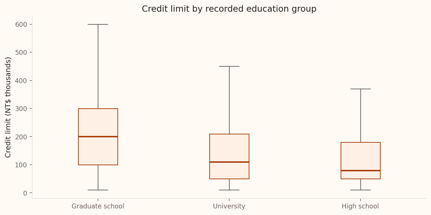
Large samples make the mean comparison stable, but Welch ANOVA or robust summaries may better address unequal spread and skew.

Source: UCI Default of Credit Card Clients. Outlier marks are hidden for legibility, not removed from analysis.

After a significant F-test

The global test does not identify differing pairs.

Use:

• prespecified contrasts;
• Tukey-adjusted pairwise comparisons;
• confidence intervals for group differences;
• an effect size such as \(\eta^2=SSG/SST\).

Under the common-variance ANOVA model, a pairwise difference has SE=sqrt(MSE(1/ni+1/nj)), with N−k error degrees of freedom. Account for the comparison family using an appropriate method such as Tukey or Bonferroni. When equal variance is doubtful, use methods compatible with unequal variances. A global test alone does not establish that every pair differs.

Complete the ANOVA reasoning

The education comparison gives \(F=1148.68\), \(p<.001\) and \(\eta^2=.072\).

1. State what the global test establishes.
2. Explain why a small p-value can coexist with 7.2% explained variation.
3. Propose a follow-up comparison and one assumption to inspect.

Allow 5 minutes within the ANOVA block before the Wooclap. At least one population mean differs under the model; this does not identify every differing pair. The large sample can make a modest association precisely detectable. Report effect size and adjusted comparisons; inspect independence, skew and differing variances. This is observational evidence, not an education intervention effect.

Read the global ANOVA result

A three-group ANOVA gives p < .001. Under the model assumptions, which conclusion follows?

1. All three pairwise differences are significant
2. At least one population mean differs; further comparisons identify which
3. Group membership causes the outcome
4. The groups have equal variances

Format: multiple choice, one answer; 90 seconds. Correct: option 2. Debrief using the credit-limit example: inspect assumptions, report effect size, and use adjusted follow-up comparisons. The observational design does not establish an education effect.

Correlation & Regression

Case: estimating a client’s bill

Question: How much can credit limit tell us about September bill amount?

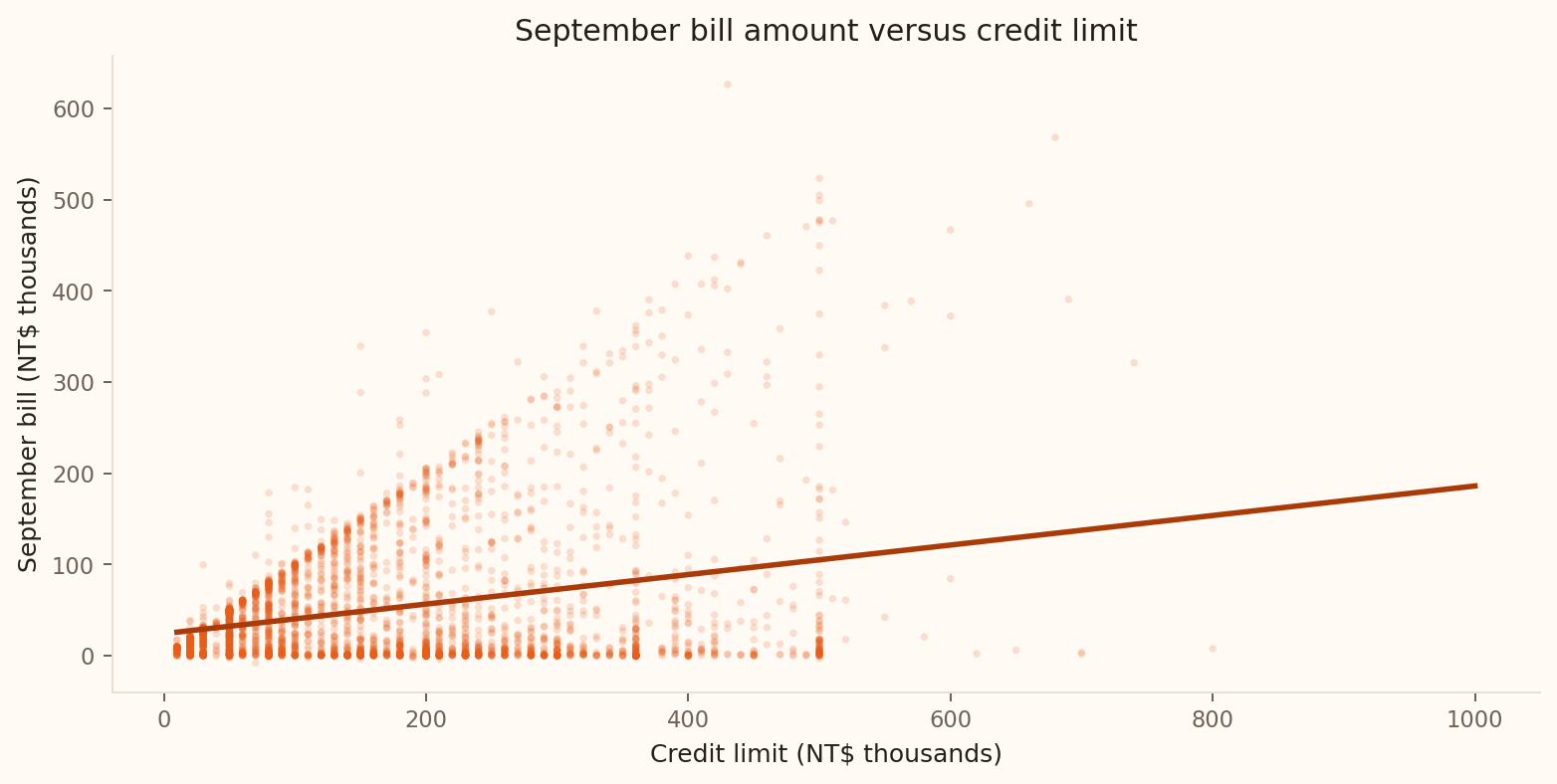
UCI Default of Credit Card Clients. Points: 3,500 sampled clients. Line: all 30,000 records. Amounts are in NT$ thousands.

Correlation

Pearson’s \(r\) summarises linear association between two numerical variables.

\[r=\frac{1}{n-1}\sum_{i=1}^n \left(\frac{x_i-\bar x}{s_x}\right) \left(\frac{y_i-\bar y}{s_y}\right)\]

\(-1\le r\le1\).

Always read direction, form, strength, and unusual observations from the scatterplot too.

Allow two minutes. Recall the visual scatterplot discussion from Week 2. Here the sample means and SDs standardise each variable, so r has no units. Both sample SDs must be positive. Paired deviations with the same sign contribute positively; deviations with opposite signs contribute negatively. Read the formula conceptually, then use r in the least-squares slope formula later in this section.

What correlation captures

\(r\)	Linear pattern
Near +1	Strong positive
Near 0	Weak or no linear pattern
Near −1	Strong negative

Correlation has no units. Shifting or rescaling by positive constants leaves it unchanged.

Allow one minute. The sign describes direction and the magnitude describes the strength of linear association. A coefficient alone cannot reveal curvature, subgroups or influential observations; the following vote and plot make this limitation visible. Changing the sign of one variable reverses the sign of r.

What does near-zero correlation mean?

For a set of loan records, Pearson’s correlation between risk score and loss is close to zero. What does this tell us about those records?

1. There is no relationship of any kind.
2. Changing the risk score cannot affect the loss.
3. There is little linear association; a curved relationship may remain.
4. The two variables are independent.

Format: multiple choice, one answer. Correct: option 3. Allow 2 minutes within the Week 8 correlation introduction: 45 seconds to vote and 75 seconds to debrief with the next slide. This is a hypothetical interpretation question about the observed records. A near-zero Pearson correlation does not establish independence or a causal conclusion. Ask students what plot they would inspect next, then show the curved pattern. The plot discussion is included in these two minutes.

What correlation misses

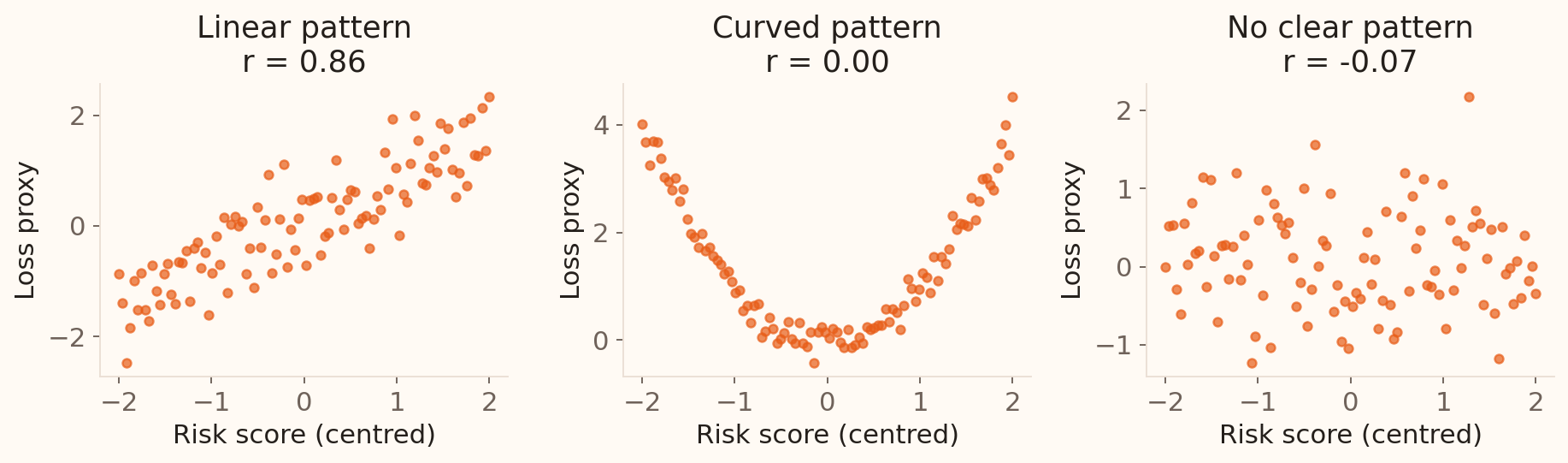
A correlation near zero can coexist with a strong curved relationship. Plots also reveal groups and influential observations.

Illustrative simulations generated in Python, seed 202602.

The population model

\[Y_i=\beta_0+\beta_1x_i+\varepsilon_i\]

Term	Meaning
\(\beta_0\)	Mean response when \(x=0\)
\(\beta_1\)	Mean response change per unit of \(x\)
\(\varepsilon_i\)	Unexplained deviation

Fitted line and residual

\[\hat y_i=b_0+b_1x_i\]

\[e_i=y_i-\hat y_i\]

Positive residual: the model underpredicts.

A fitted value lies on the line; a residual is the observation’s signed vertical distance from it.

Fit the line by least squares

Choose \(b_0,b_1\) to minimise

\[SSE=\sum_{i=1}^n(y_i-\hat y_i)^2=\sum e_i^2.\]

Squaring prevents cancellation and penalises large errors.

\[b_1=r\frac{s_y}{s_x},\qquad b_0=\bar y-b_1\bar x.\]

The fitted line passes through \((\bar x,\bar y)\), and the slope has units “response per predictor unit”.

Interpret in context

With bill amount measured in thousand NTD and credit limit in 10,000 NTD:

\[\widehat{\text{bill}}=24.09+1.620(\text{credit limit}).\]

Each additional 10,000 NTD of credit limit is associated with an estimated 1,620 NTD higher mean September bill.

This is an association across observed accounts, not a lending-policy effect.

Interpret the slope with units

Bill is measured in thousand NTD and credit limit in units of 10,000 NTD. The fitted slope is 1.620. What does it describe?

1. An associated mean bill increase of 1,620 NTD per extra 10,000 NTD of credit limit
2. A guaranteed 1,620 NTD increase for every client
3. A causal increase of 16,200 NTD
4. A 162% increase in default risk

Format: multiple choice, one answer; 90 seconds. Correct: option 1. Debrief: attach both units to the coefficient; it concerns the conditional mean in an observational relationship, not each individual outcome or a causal policy effect.

Prediction & Inference

Keep the data range in view

Observed credit limits range from 10,000 to 1,000,000 NTD.

Prediction point	Interpretation
Zero limit	The intercept is a fitted baseline outside the observed range
200,000 NTD	Within the observed range
2,000,000 NTD	Extrapolation; a new lending policy or customer group may behave differently

Use the intercept to define the line; assess whether it has a meaningful practical interpretation.

Prediction

At \(x_0\):

\[\hat y_0=b_0+b_1x_0.\]

Mean-response interval

Uncertainty about \(E(Y\mid x_0)\)

Prediction interval

Uncertainty for one new \(Y\)

Prediction intervals are wider.

At a 200,000 NTD credit limit, the fitted mean bill is 56,491 NTD.

Under the usual linear model, a mean-response interval uses SE=s_e sqrt(1/n+(x0−xbar)^2/Sxx). An individual prediction interval adds 1 inside that square root, accounting for new-observation variation. Both are conditional on the model being suitable and are wider away from xbar. The real bill residuals later show why these assumptions need inspection.

Decomposing variation

\[SST=SSR+SSE\]

Quantity	Meaning
\(SST=\sum(y_i-\bar y)^2\)	Total variation
\(SSR=\sum(\hat y_i-\bar y)^2\)	Explained variation
\(SSE=\sum(y_i-\hat y_i)^2\)	Residual variation

How much variation does the model explain?

\[R^2=\frac{SSR}{SST}=1-\frac{SSE}{SST}.\]

Here \(R^2=.0815\): credit limit explains 8.15% of observed September-bill variation in the fitted linear model.

For simple regression with an intercept, \(R^2=r^2\). Here \(r=.285\) indicates a positive, weak linear association.

Pearson r ranges from −1 to 1 and retains direction. In-sample R-squared for OLS with an intercept ranges from zero to one and measures explained variation. With several predictors there is no single predictor correlation whose square gives the model R-squared. Test-set R-squared can be negative. Assess prediction using held-out observations; fit alone does not establish causality.

LINE conditions

Linear

Mean pattern

Independent

Errors across units

Normal

Errors for exact inference

Equal variance

Across fitted values

These are assumptions about the model errors, assessed using residuals and the study design. E(error|X)=0 is needed for the usual conditional mean interpretation. Error normality supports exact small-sample t and F inference; it is not required merely to calculate least squares. Equal variance is needed for the conventional SE formulas used here.

Testing the slope

\[H_0:\beta_1=0 \qquad H_A:\beta_1\ne0\]

\[t=\frac{b_1}{SE(b_1)},\qquad df=n-2\]

This tests for a population linear association.

For the credit-limit slope:

\[t=51.58,\qquad df=29{,}998,\qquad p<.001.\]

Quantify the slope uncertainty

\[b_1\pm t^*_{n-2}SE(b_1).\]

Quantity	NTD per extra 10,000 NTD of credit limit
Estimated slope	1,620
Conventional standard error	31.4
Model-based 95% interval	1,558 to 1,681

Check the model conditions before relying on this interval.

Use about 3 minutes in the slope-inference block. The standard error formula and residual-SD calculation are retained in the reference slide. Interpret this as an interval for the mean association, not individual bills or a policy effect. The next residual plot shows why conventional equal-variance standard errors need scrutiny.

Residuals versus fitted

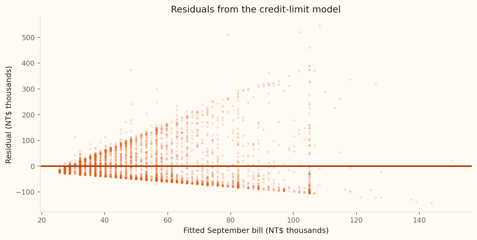
Address the changing residual spread before trusting model intervals.

Source: UCI Default of Credit Card Clients. Plot shows a reproducible 4,500-record sample of residuals from the all-record fit.

A First Multiple Model

Add predictors carefully

\[Y=\beta_0+\beta_1X_1+\cdots+\beta_pX_p+\varepsilon\]

Multiple regression describes conditional associations, holding included predictors fixed. Causal interpretation also needs an appropriate design.

Categorical predictors

Group September repayment status and choose no recorded delay as the reference:

Status	One-month indicator	Two-or-more-months indicator
No recorded delay	0	0
One month late	1	0
Two or more months late	0	1

Each indicator coefficient compares that group with the reference, holding other predictors fixed.

The grouping uses PAY_0 <= 0, PAY_0 == 1, and PAY_0 >= 2. It avoids treating all numeric status codes as equally spaced measurements. An intercept plus k−1 indicators represents k categories; including all k indicators and an intercept creates exact collinearity.

Multiple-regression output

Predictor	Estimate	SE	p-value
Intercept	19.888	1.654	<.001
Limit (per 10,000 NTD)	1.659	0.032	<.001
Age (years)	0.111	0.044	.012
One month late	−21.368	1.242	<.001
Two or more months late	21.315	1.349	<.001

Adjusted \(R^2=.101\). An extra 10,000 NTD of limit is associated with 1,659 NTD higher mean bill, holding age and status group fixed.

UCI credit data, all 30,000 records. Bill and coefficients are in thousand NTD; conventional OLS standard errors.

The one-month and two-or-more-month coefficients compare each group with no recorded delay at the same credit limit and age. Their signs need not follow a monotonic progression. These conditional associations can reflect billing behaviour and customer composition. Recheck residuals for this expanded model before relying on conventional inference or using predictions.

Session 8 takeaway

• ANOVA tests a global difference; adjusted comparisons locate it.
• Least squares fits a line by minimising squared residuals.
• Interpret slopes with units and check the conditions for inference.
• Multiple-regression coefficients hold included predictors fixed.

Next: examine model behaviour, compare alternatives and complete a banking analysis.

Reference

Slope uncertainty and interpretation

\[SE(b_1)=\frac{s_e} {\sqrt{\sum(x_i-\bar x)^2}},\]

where

\[s_e=\sqrt{\frac{SSE}{n-2}}.\]

The interval is \(b_1\pm t^*_{n-2}SE(b_1)\).

Here \(SE(b_1)=31.4\) NTD per 10,000 NTD of limit; the model-based 95% interval is 1,558 to 1,681 NTD higher mean bill.

These are conventional homoskedastic OLS standard errors. More data, wider predictor spread, and lower residual noise improve precision under the model. The core residual plot in this session shows changing spread; Session 9 develops the diagnostics and possible responses.

Write the regression finding

For credit limit and September bill amount:

• Estimated bill increase per extra 10,000 NTD of limit: 1,620 NTD.
• Model-based 95% interval: 1,558 to 1,681 NTD; \(p<.001\).
• \(R^2=.0815\); residual spread changes with fitted bill amount.

Write three sentences covering association, usefulness for prediction, and the next analytical check.

Optional follow-up exercise, outside the core timetable. Allow 12 minutes if used: 5 minutes drafting in pairs, 5 minutes comparing answers, 2 minutes debrief. Example: A higher limit is associated with a higher mean bill, with estimated slope 1,620 NTD per 10,000 NTD of limit. Credit limit alone explains 8.15% of observed variation, so significance does not establish accurate individual predictions. Examine the changing residual spread and use an appropriate model or standard-error method before relying on conventional intervals, then assess predictions on held-out data. Session 9 develops the diagnostic and validation workflow.

Inference for one variance

For normal data,

\[\frac{(n-1)s^2}{\sigma_0^2}\sim\chi^2_{n-1}.\]

This gives tests and confidence intervals for a population variance. The method is sensitive to non-normality.

A 95% interval is \([(n-1)s^2/q_{.975},\ (n-1)s^2/q_{.025}]\), where \(q_u\) is the \(u\) quantile of \(\chi^2_{n-1}\).

Comparing two variances

For independent normal samples under \(H_0:\sigma_1^2=\sigma_2^2\),

\[F=\frac{s_1^2}{s_2^2}\sim F_{n_1-1,n_2-1}.\]

In routine mean comparisons, Welch’s method is usually preferable to testing variances first.