Modelling numerical variables
In this unit we will learn to quantify the relationship between two numerical variables, as well as modelling numerical response variables using a numerical or categorical explanatory variable.
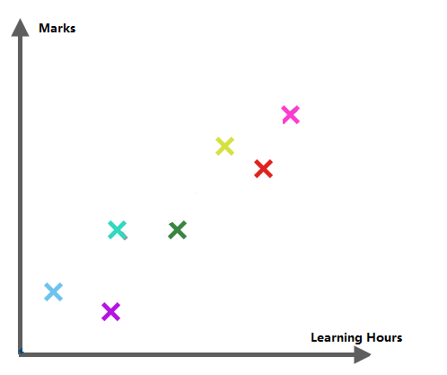
Learning Hours vs Exam Marks
What can we observe from the scatter plot?
Explanatory Variable: Learning Hours
Response Variable: Final Exam Marks
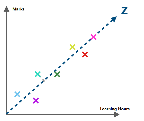
Relationship: Linear positive, strong
How to capture the relationship? \[\hat{y} = \beta_0 + \beta_1 x\]
Residuals
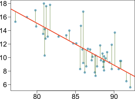
Residuals are the leftovers from the model fit: Data = Fit + Residual
Residuals (cont.)
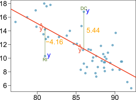
Residual Residual is the difference between the observed (\(y_i\)) and predicted \(\hat{y}_i\). \[e_i = y_i - \hat{y}_i\]
Quantifying the relationship
Correlation describes the strength of the linear association between two variables.
It takes values between -1 (perfect negative) and +1 (perfect positive).
A value of 0 indicates no linear association.
Assessing the correlation
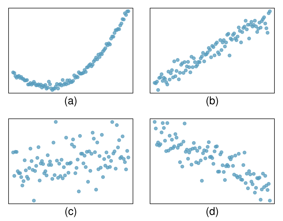
Which of the following is has the strongest correlation, i.e. correlation coefficient closest to +1 or -1?
(b) correlation means linear association
The least squares line
\[ \hat{y} = \beta_0 + \beta_1 x \]
\(\hat{y}\): Predicted value of the response variable, \(y\)
\(\beta_0\): Intercept, parameter
- \(b_0\): Intercept, point estimate
\(\beta_1\): Slope, parameter
- \(b_1\): Slope, point estimate
\(x\): Explanatory variable
Conditions for the least squares line
Linearity
Nearly normal residuals
Constant variability
Conditions: (1) Linearity
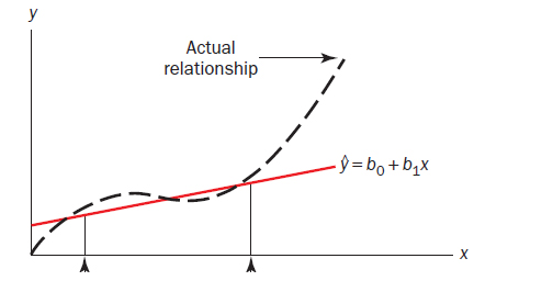
The relationship between the explanatory and the response variable should be linear.
Methods for fitting a model to non-linear relationships exist, but are beyond the scope of this class.
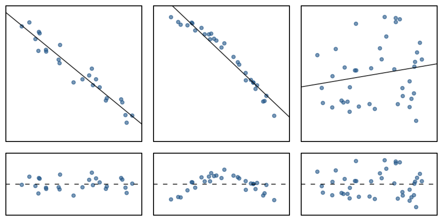
Check using a scatterplot of the data or residuals plot.
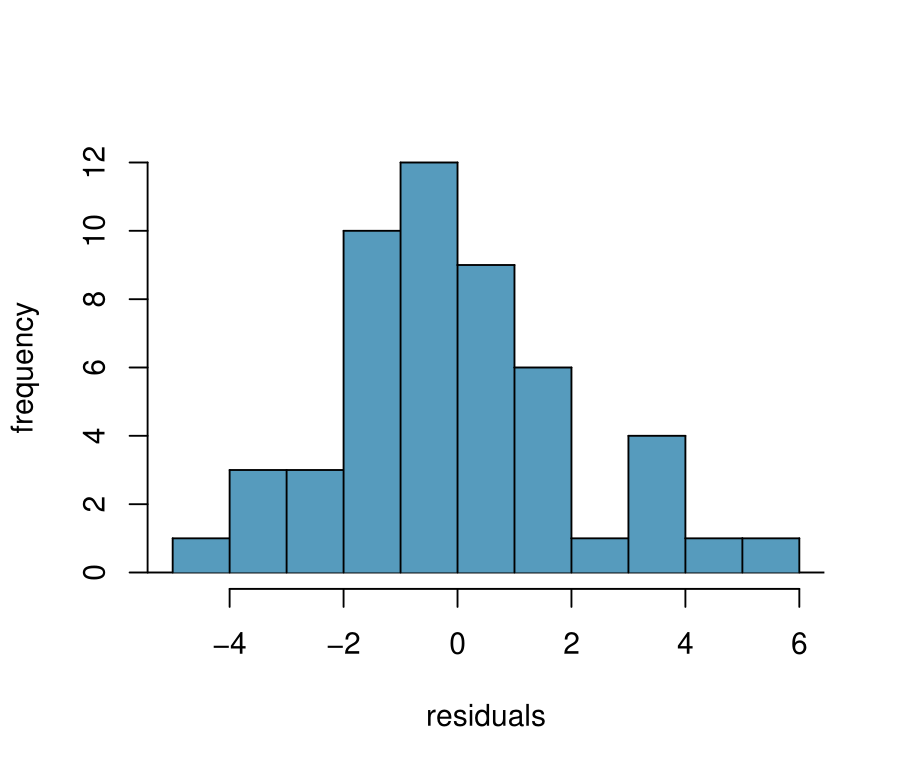
Conditions: (2) Nearly normal residuals
Conditions: (3) Constant variability
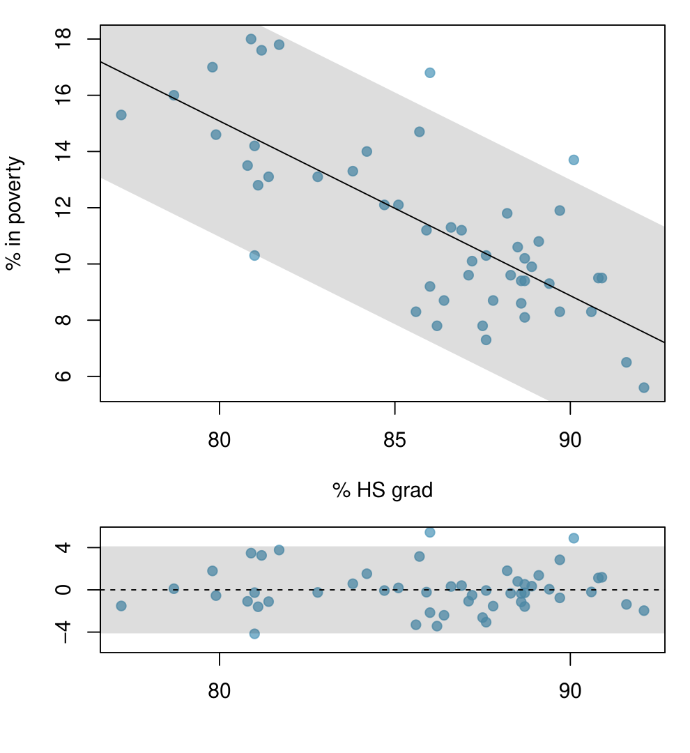
The variability of points around the least squares line should be roughly constant.
This implies that the variability of residuals around the 0 line should be roughly constant as well.
Also called homoscedasticity.
Check using a residual plot (The residual plot should give an overall impression of a horizontal band of points).
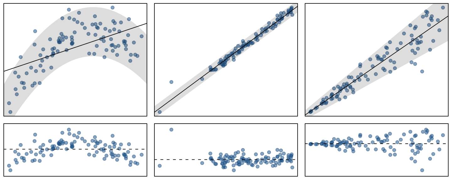
Checking conditions
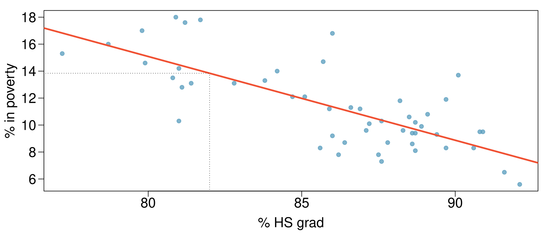
What condition is this linear model obviously violating?
Constant variability
Linear relationship
Normal residuals
No extreme outliers
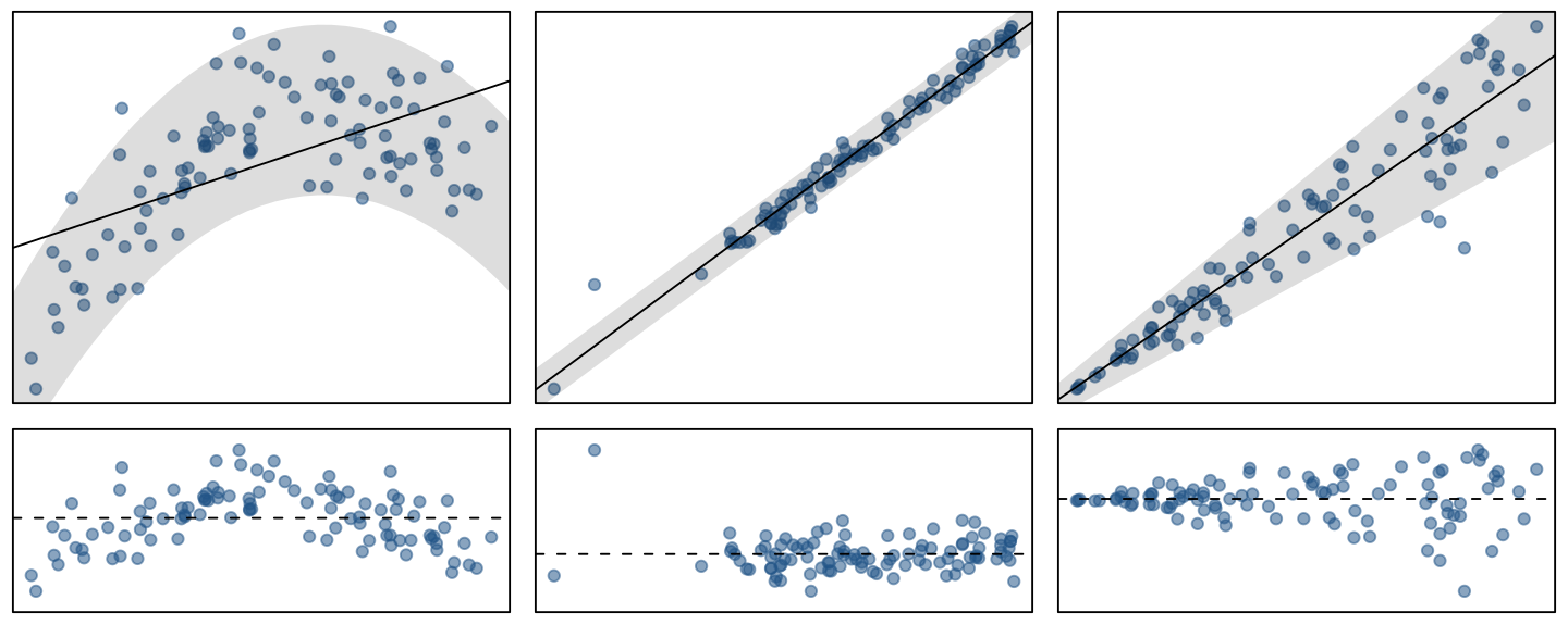
Checking conditions
What condition is this linear model obviously violating?
Constant variability
Linear relationship
Normal residuals
No extreme outliers
Summarise conditions
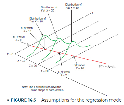
Since the existence residual, our regression model is indeed: \[Y = \beta_0 + \beta_1 x + \varepsilon\] where \(\varepsilon\) can be used as the residual term, which is assumed to follow: \[\varepsilon \sim N(0, \sigma^2).\] That is to say,
The expected residual is 0, \(E(\varepsilon) = 0\), thus \(E(Y) = \beta_0 + \beta_1 x\)
Variance of residual is \(\sigma^2\), thus it is a constant
For each observation, the residual has the same distribution, but independent, (i.i.d), identically independent distributed.
Therefore, we can have
\(Y|x = constant + \varepsilon \sim N(\text{constant}, \sigma^2)\)
Given a specific \(x\), Y is normally distributed random variable.
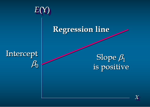
Estimated Simple Linear Regression Equation
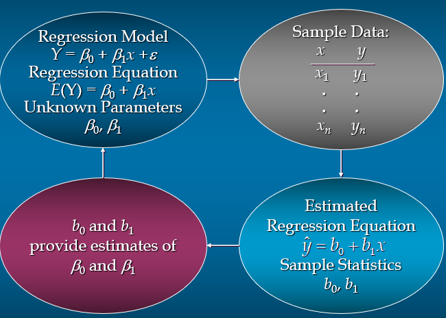
The estimated simple linear regression equation \[\hat{y} = b_0 + b_1x\]
The graph is called the estimated regression line.
\(b_0\) is the intercept of the line.
\(b_1\) is the slope of the line.
\(\hat{y}\) is the estimated value of \(Y\) for a given \(x\) value.
Estimation of \(b_0\) and \(b_1\)
Least Squares Criterion \[\min \sum (y_i - \hat{y}_i)^2 = \min \sum (y_i - b_0 - b_1 x_i)^2\] where:
Derivative with respect to \(b_1\) =0 and then solve the equation \[b_1 = \frac{\sum (x_i - \bar{x})(y_i - \bar{y})}{\sum (x_i - \bar{x})^2}, \quad b_0 = \bar{y} - b_1\bar{x}\]
\(x_i\) = value of independent variable for \(i\)th observation
\(y_i\) = value of dependent variable for \(i\)th observation
\(\bar{x}\) = mean value for independent variable
\(\bar{y}\) = mean value for dependent variable
\(n\) = total number of observations
Interpretation of slope and intercept
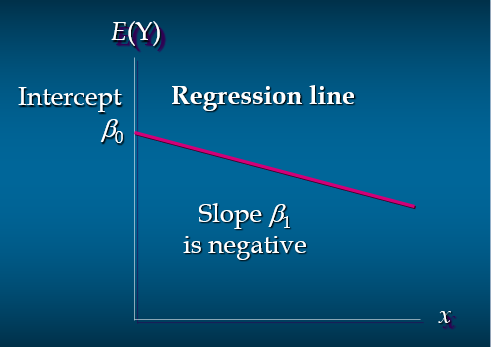
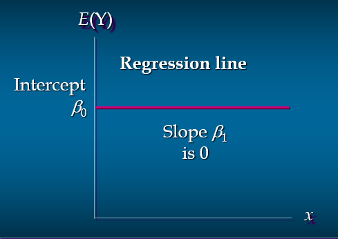
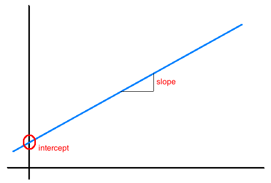
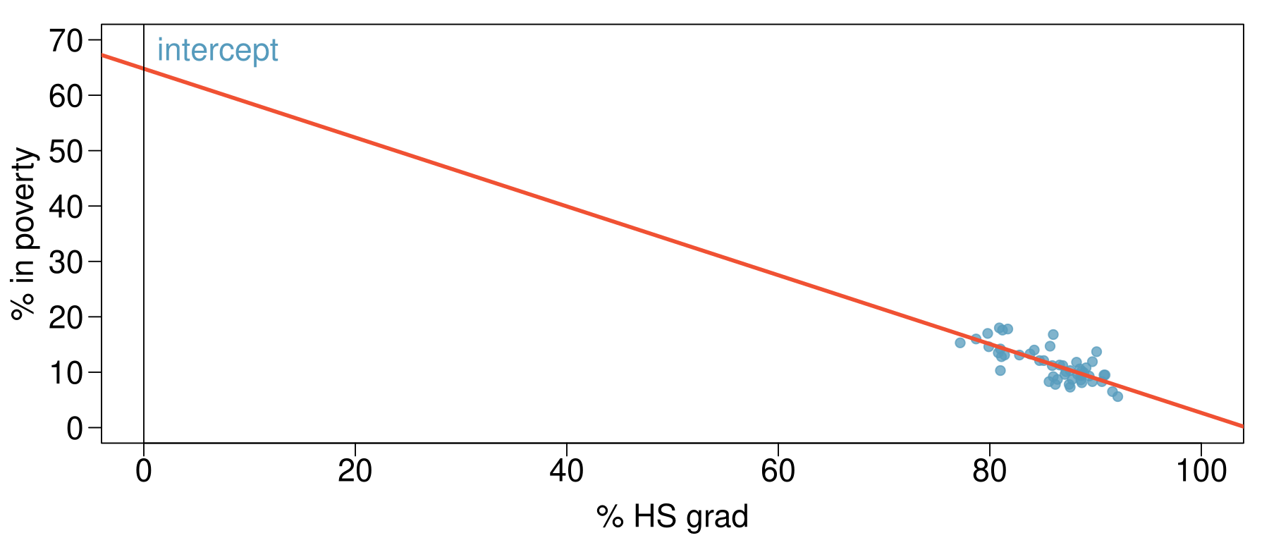
Intercept: When \(x = 0\), \(y\) is expected to equal the intercept.
\(\:\)
Slope: For each unit in \(x\), \(y\) is expected to increase / decrease on average by the slope.
These statements are not causal, unless the study is a randomised controlled experiment.
Prediction
Using the linear model to predict the value of the response variable for a given value of the explanatory variable is called prediction, simply by plugging in the value of \(x\) in the linear model equation.
There will be some uncertainty associated with the predicted value.
Coefficient of Determination
Relationship Among SST, SSR, SSE \[\text{SS}_{tot} = \text{SS}_{reg} + \text{SS}_{res}\] \[\sum (y_i - \bar{y})^2 = \sum (\hat{y}_i - \bar{y})^2 + \sum (y_i - \hat{y}_i)^2\]
where:
\(\text{SS}_{tot}\) = total sum of squares
\(\text{SS}_{reg}\) = sum of squares due to regression
\(\text{SS}_{res}\) = sum of squares due to error
\(R^2\) (Coefficient of Determination)
Formula: \(R^2 = \frac{\text{SS}_{reg}}{\text{SS}_{tot}}=1 - \frac{\text{SS}_{\text{res}}}{\text{SS}_{\text{tot}}}\)
Represents the proportion of variance in the dependent variable that’s predictable from the independent variables.
Measures the goodness of fit of a regression model.
Pearson Correlation Coefficient
Sample Variance of \(X\) \[s_{x}^2 = \frac{\sum (x_i - \bar{x})^2}{n - 1} = \frac{\sum (x_i - \bar{x})(x_i - \bar{x})}{n - 1}\]
Covariance \[s_{xy} = \frac{\sum (x_i - \bar{x})(y_i - \bar{y})}{n - 1} \quad \text{for samples}, \quad
\sigma_{xy} = \frac{\sum (x_i - \mu_x)(y_i - \mu_y)}{N} \quad \text{for populations}\]
Pearson Correlation Coefficient \[r_{xy} = \frac{s_{xy}}{s_x s_y} \quad \text{for samples}, \quad \rho_{xy} = \frac{\sigma_{xy}}{\sigma_x \sigma_y} \quad \text{for populations}\]
Computational Formula \[r = \frac{\sum (x_i - \bar{x})(y_i - \bar{y})}{\sqrt{(\sum x_i^2 - n(\bar{x})^2)(\sum y_i^2 - n(\bar{y})^2)}} =\frac{\sum x_i y_i - n \bar{x} \bar{y}}{\sqrt{(\sum x_i^2 - n(\bar{x})^2)(\sum y_i^2 - n(\bar{y})^2)}}\]
Pearson Correlation Coefficient
\(r = r_{xy} = \frac{\sum (x_i - \bar{x})(y_i - \bar{y})}{\sqrt{(\sum x_i^2 - n(\bar{x})^2)(\sum y_i^2 - n(\bar{y})^2)}} =\frac{\sum x_i y_i - n \bar{x} \bar{y}}{\sqrt{(\sum x_i^2 - n(\bar{x})^2)(\sum y_i^2 - n(\bar{y})^2)}}\)
Indicates the proportion of variance in one variable that is predictable from the another variable.
Therefore, the correlation coefficient is particularly helpful in assessing and managing investment risks.
The modern portfolio theory suggests diversification can reduce the volatility of a portfolio’s returns, curbing risk
The correlation coefficient between historical returns can indicate whether adding an investment to a portfolio will improve its diversification.
Difference Between \(R^2\) and \(r^2\)
\(R^2\) (Coefficient of Determination)
Formula: \(R^2 = 1 - \frac{\text{SS}_{\text{res}}}{\text{SS}_{\text{tot}}} = \frac{\sum (\hat{y}_i - \bar{y})^2}{\sum (y_i - \bar{y})^2 }\)
Represents the proportion of variance in the dependent variable that’s predictable from the independent variables.
Measures the goodness of fit of a regression model.
\(r^2\) (Squared Pearson Correlation Coefficient)
Formula: \(r^2 = \left( \frac{\sum (x_i - \bar{x})(y_i - \bar{y})}{\sqrt{\sum (x_i - \bar{x})^2 \sum (y_i - \bar{y})^2}} \right)^2\)
Indicates the proportion of variance in one variable that is predictable from the other variable.
In simple linear regression, they’re identical because: \[\begin{aligned}
R^2 &= \frac{\sum (\hat{y}_i - \bar{y})^2}{\sum (y_i - \bar{y})^2 } = \frac{\sum (b_0 + b_1 x_i - \bar{y})^2}{\sum (y_i - \bar{y})^2 } = \frac{\sum (\bar{y} - b_1 \bar{x} + b_1 x_i - \bar{y})^2}{\sum (y_i - \bar{y})^2 } = \frac{b_1^2 \sum (x_i - \bar{x})^2}{\sum (y_i - \bar{y})^2 } \\
& = \left(\frac{\sum (x_i - \bar{x})(y_i - \bar{y})}{\sum (x_i - \bar{x})^2} \right)^2 \times \frac{\sum (x_i - \bar{x})^2}{\sum (y_i - \bar{y})^2 } = r^2
\end{aligned}\]
\(R^2\) vs \(r\)
\(R^2\)
It tells us what percent of variability in the response variable is explained by the model.
It is used to measure the goodness of fit of regression model, not only linear regression model.
\(r\)
- It is used to measure the correlation between two variables, no only in the regression analysis.
Interpretation of \(R^2\)
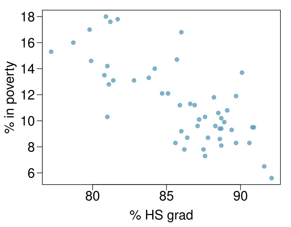
Which of the below is the correct interpretation of \(r = -0.75\), \(R^2 = 0.56\)?
56% of the variability in the % of HG graduates is explained by the model.
56% of the variability in the % of residents living in poverty is explained by the model.
56% of the time % HS graduates predict % living in poverty correctly.
75% of the variability in the % of residents living in poverty is explained by the model.
Types of outliers
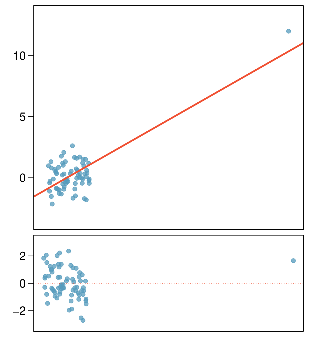
How do outliers influence the least squares line in this plot?
To answer this question think of where the regression line would be with and without the outlier(s).
Without the outliers the regression line would be steeper, and lie closer to the larger group of observations.
With the outliers the line is pulled up and away from some of the observations in the larger group.
Types of outliers
How do outliers influence the least squares line in this plot?
Without the outlier there is no evident relationship between \(x\) and \(y\).
Some terminology
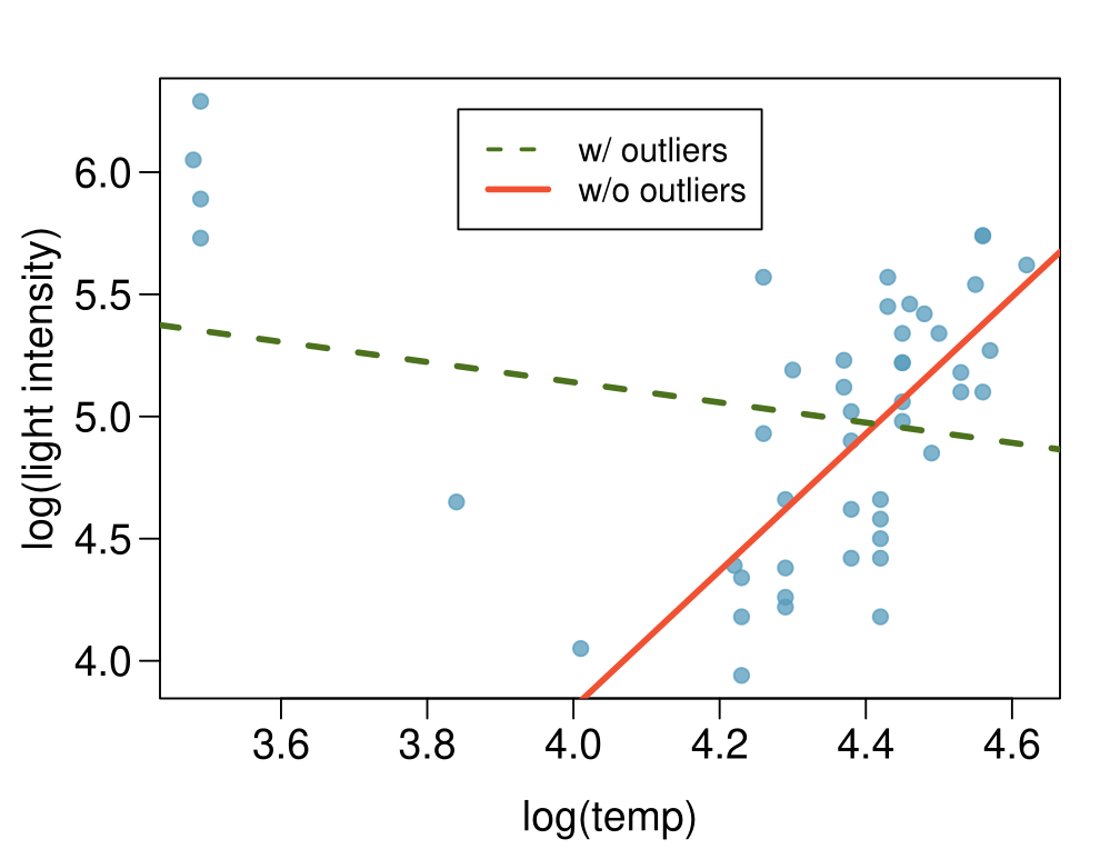
Outliers are points that lie away from the cloud of points.
Outliers that lie horizontally away from the centre of the cloud are called high leverage points.
High leverage points that actually influence the slope of the regression line are called influential points.
In order to determine if a point is influential, visualise the regression line with and without the point. Does the slope of the line change considerably? If so, then the point is influential. If not, then it’s not an influential point.
Influential points
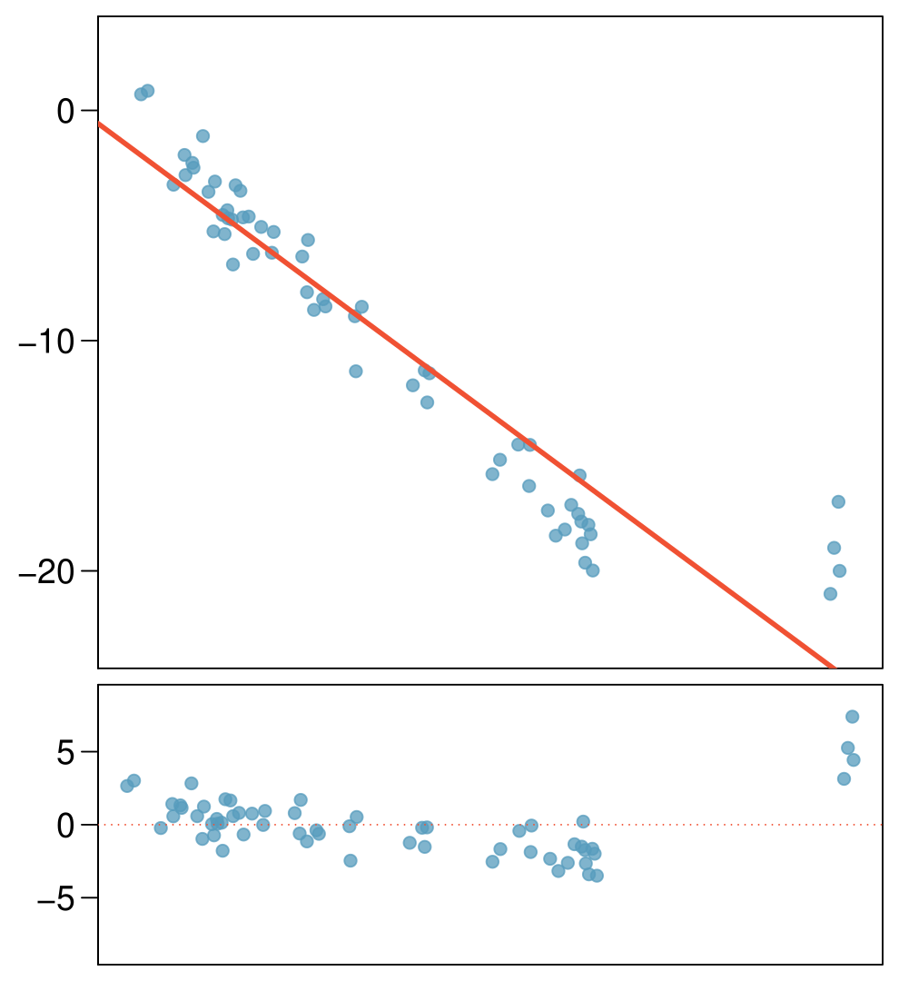
Data are available on the log of the surface temperature and the log of the light intensity of 47 stars in the star cluster CYG OB1.
Types of outliers
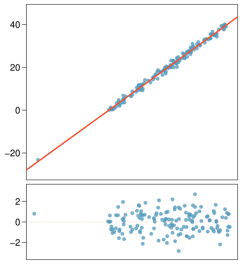
Which of the below best describes the outlier?
influential
high leverage
none of the above
there are no outliers
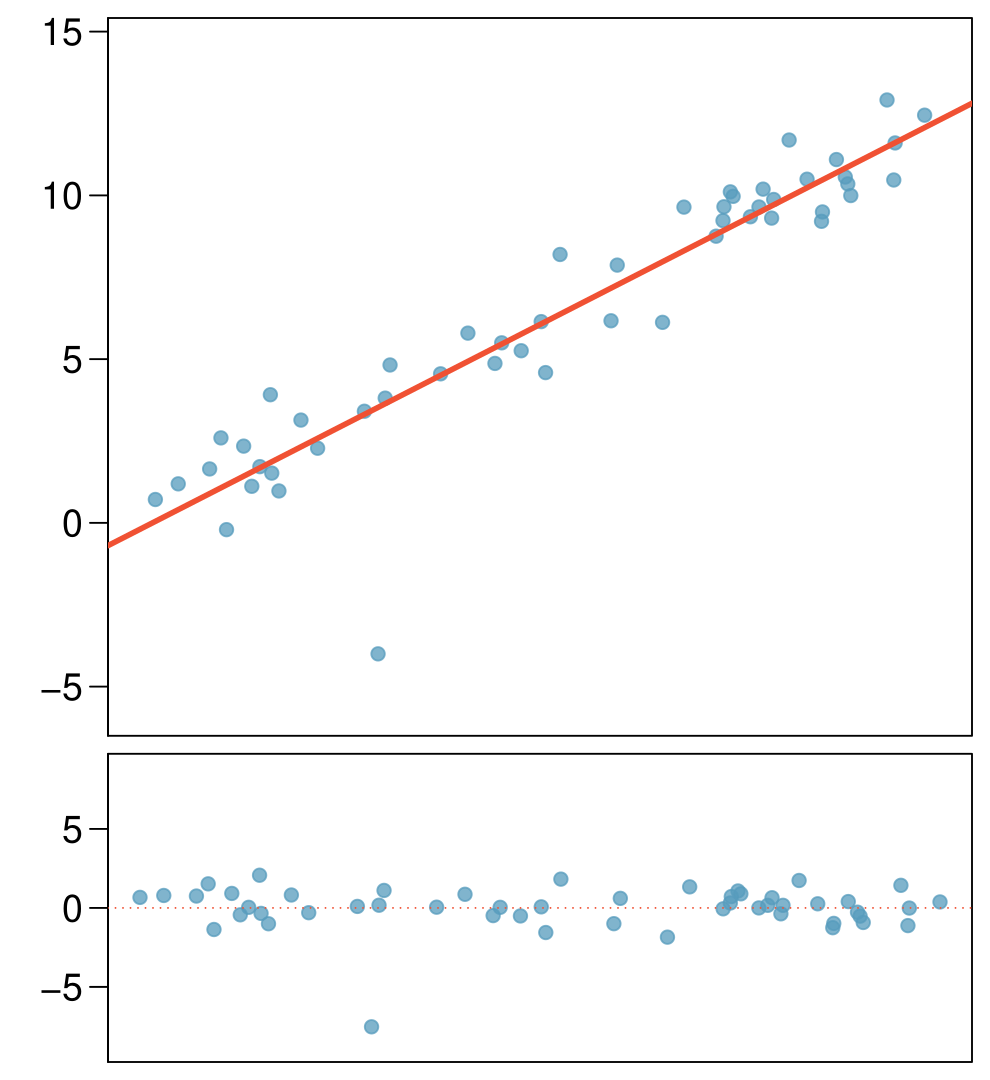
Types of outliers
Does this outlier influence the slope of the regression line? Not much...
Recap
Which of following is true?
Influential points always change the intercept of the regression line.
Influential points always reduce \(R^2\).
It is much more likely for a low leverage point to be influential, than a high leverage point.
When the data set includes an influential point, the relationship between the explanatory variable and the response variable is always nonlinear.
None of the above.
Testing for Significance
To test for a significant regression relationship, we must conduct a hypothesis test to determine whether the value of \(\beta_1\) is zero.
Testing for the slope
In simple linear regression, we model the relationship between a dependent variable \(Y\) and an independent variable \(X\) as: \[Y = \beta_0 + \beta_1X + \varepsilon\]
Where:
Which hypothesis is TRUE?
\(H_0:\) \(b_0 = 0\); \(H_1:\) \(b_0 \ne 0\)
\(H_0:\) \(\beta_0 = 0\); \(H_1:\) \(\beta_0 \ne 0\)
\(H_0:\) \(b_1 = 0\); \(H_1:\) \(b_1 \ne 0\)
\(H_0:\) \(\beta_1 = 0\); \(H_1:\) \(\beta_1 \ne 0\)
Testing for Significance: Procedure
Estimate the regression model to obtain \(\hat{\beta}_1 = b_1 = \frac{\sum (x_i - \bar{x})(y_i - \bar{y})}{\sum (x_i - \bar{x})^2}\).
Calculate the t-statistic: \[t = \frac{b_1 - 0}{SE(b_1)}\]
Decide based on the critical value or p-value (preferred). \[p-value = \mathbb{P}(| t | > t_{statistic}) < \alpha\]
Calculating \(SE(\hat{\beta}_1)\)
SE of the Estimated Slope
Steps to Calculate \(SE(b_1)\):
Calculate the SSE: \[SSE = \sum (y_i - \hat{y}_i)^2\]
Estimate the variance of the error term: \[\hat{\sigma}^2 = \frac{SSE}{n-2}\]
Finally, compute \(SE(\hat{\beta}_1)\): \[SE(b_1) = \sqrt{\frac{\hat{\sigma}^2}{\sum (x_i - \bar{x})^2}}\]
Note 1: \[\begin{aligned}
b_1 & = \frac{\sum (x_i - \bar{x})(y_i - \bar{y})}{\sum (x_i - \bar{x})^2}
= \frac{\sum (x_i - \bar{x})(\beta_1 x_i + \beta_0 + \varepsilon - \bar{y})}{\sum (x_i - \bar{x})^2}
= \frac{\sum (x_i - \bar{x})(\beta_1 x_i + \bar{y} - \beta_1 \bar{x} + \varepsilon - \bar{y})}{\sum (x_i - \bar{x})^2} \\
&= \beta_1 + \frac{\sum (x_i - \bar{x}) \varepsilon}{\sum (x_i - \bar{x})^2}
\sim N\left(\beta_1, \frac{\sigma^2}{\sum (x_i - \bar{x})^2}\right)
\end{aligned}\] Note 2: We lose 1 degree of freedom for each parameter we estimate, and in simple linear regression we estimate 2 parameters, \(\beta_0\) and \(\beta_1\).
Confidence Interval for \(\beta_1\)
The form of a confidence interval for \(\beta_1\) is \[b_1 \pm t_{\alpha/2} \times \text{SE}(b_1)\]
\(b_1\) is the point estimator
The t-distribution has the degree of freedom n-2
CI = 1 - \(\alpha\)
\(H_0\) is rejected if the hypothesised value of \(\beta_1\) (usually it is 0) is not included in the confidence interval for \(\beta_1\).
Recap
Inference for the slope for a single-predictor linear regression model:
Hypothesis test: \[T = \frac{b_1 - null~value}{SE(b_1)} \qquad df = n - 2\]
Confidence interval: \[b_1 \pm t^\star_{df = n - 2, \alpha/2} SE(b_1)\]
The null value is often 0 since we are usually checking for any relationship between the explanatory and the response variable.
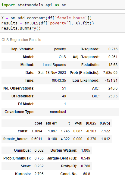
The regression output gives \(b_1\), \(SE_{b_1}\), and two-tailed p-value for the \(t\)-test for the slope where the null value is 0.
We rarely do inference on the intercept, so we’ll be focusing on the estimates and inference for the slope.
Some cautions about the interpretation
In addition, just because we are able to reject \(H_0: \beta_1 = 0\) and demonstrate statistical significance it does NOT enable us to conclude that the relationship between X and Y is linear.
We can state only that X and Y are related and that a linear relationship explains a significant proportion of the variability in Y over the range of values for X observed in the sample.
Multiple Linear Regression
Multiple regression
Simple linear regression: Bivariate - two variables: \(y\) and \(x\)
Multiple linear regression: Multiple variables: \(y\) and \(x_1, x_2, \cdots\)
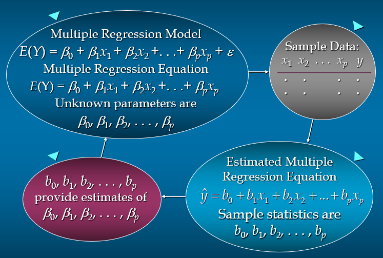
The equation that describes how the dependent variable \(Y\) is related to the independent variables \(X_1, X_2, \ldots, X_p\) and an error term is called the multiple regression model.
\[Y = \beta_0 + \beta_1 X_1 + \beta_2 X_2 + \ldots + \beta_p X_p + \varepsilon\]
where:
\(\beta_0, \beta_1, \beta_2, \ldots, \beta_p\) are the parameters,
\(X_1, X_2, \ldots, X_p\) are the independent variables,
\(\varepsilon\) is a random variable called the error term.
Multiple Regression Equation
The equation that describes how the mean value of \(Y\) is related to \(X_1, X_2, \ldots, X_p\) is called the multiple regression equation.
\[E(Y) = \beta_0 + \beta_1 X_1 + \beta_2 X_2 + \ldots + \beta_p X_p\]
Estimated Multiple Regression Equation
A simple random sample is used to compute sample statistics \(b_0, b_1, b_2, \ldots, b_p\) that are used as the point estimators of the parameters \(\beta_0, \beta_1, \beta_2, \ldots, \beta_p\). The estimated multiple regression equation is:
\[\hat{y} = b_0 + b_1 X_1 + b_2 X_2 + \ldots + b_p X_p\]
Multiple Regression Graph
How to Estimate the Coefficient Value?
\[\min \sum(y_i - \hat{y}_i)^2\]
The formulas for the regression coefficients are very complicated (needs knowledge of matrix algebra), so we will always use Software to perform the calculations.
We will show it later
Testing for Significance
Hypotheses \(H_0: \beta_1 = \beta_2 = \ldots = \beta_p = 0\)
\(H_1\): At least one \(\beta_i\) is not equal to zero.
Test Statistic \[F = \frac{MSR}{MSE}\] Where MSR (SSR/p) is the mean square regression and MSE (SSE / (n-p-1)) is the mean square error.
Rejection Rule Reject \(H_0\) if \(p\text{-value} \leq \alpha\) or if \(F > F_{\alpha}\),
where \(F_{\alpha}\) is the critical value from the F distribution with \(p\) degrees of freedom in the numerator and \(n - p - 1\) degrees of freedom in the denominator.
Dummy Variables
Dummy variables allow us to include categorical predictors in a regression model.
For a categorical variable with \(k\) categories, we create \(k-1\) dummy variables.
Each dummy variable represents one category and takes the value 1 if an observation belongs to that category, and 0 otherwise.
The category not represented by its own dummy variable is considered the baseline and is represented by all dummy variables being 0.
In the regression equation, each dummy variable has its own coefficient, which measures the effect of that category relative to the baseline.
Example of Dummy Variables
Original categorical data: Preferred Banking Service (Online, In-Branch, Mobile App)
Two dummy variables: Service_Online, Service_InBranch (with Mobile App as the baseline)
Example Data from Banking Sector and Corresponding Dummy Variables
| Online |
1 |
0 |
| In-Branch |
0 |
1 |
| Mobile App |
0 |
0 |
| Online |
1 |
0 |
| Mobile App |
0 |
0 |
| In-Branch |
0 |
1 |
Each row represents a customer’s preference for a banking service.
Service_Online and Service_InBranch are dummy variables indicating the preference.
Mobile App, not having a dedicated dummy variable, serves as the baseline.
Interpreting Coefficients with Dummy Variables
Model Equation Customer_Satisfaction = \(\beta_0\) + \(\beta_1\) * Service_Online + \(\beta_2\) * Service_InBranch + \(\varepsilon\)
Interpreting Coefficients
\(\beta_1\) (Service_Online): The change in customer satisfaction score when using online banking compared to mobile app banking.
\(\beta_2\) (Service_InBranch): The change in customer satisfaction score when using in-branch banking compared to mobile app banking.
Note: The baseline (Mobile App) is implied when both dummy variables are 0.
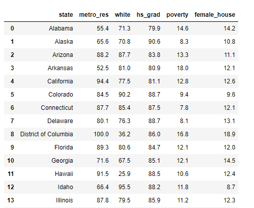
Example: Modelling Poverty
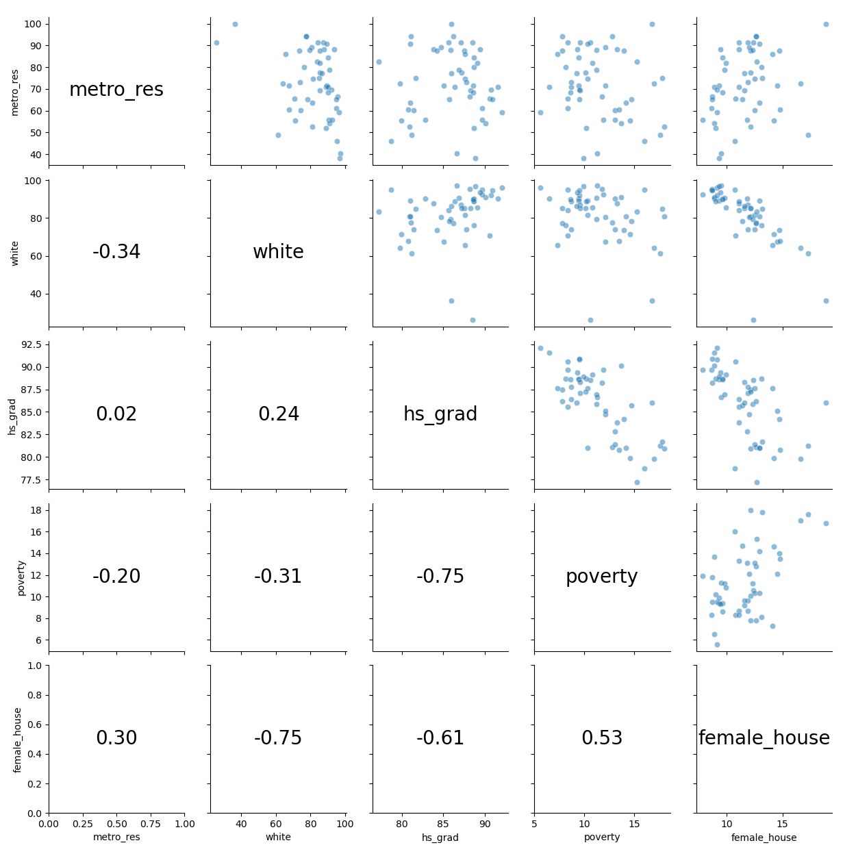
Correlation and Scatterplot
Look at \(R^2\)
\(R^2\) can be calculated as the definition,
\[R^2 = 1 - \frac{\text{SS}_{E}}{\text{SS}_{tot}} = \frac{\text{explained variability in }y}{\text{total variability in }y}\]
Using ANOVA we can calculate the explained variability and total variability in \(y\).
Sum of squares
| female_house |
1 |
132.57 |
132.57 |
18.68 |
0.00 |
| Residuals |
49 |
347.68 |
7.10 |
|
|
| Total |
50 |
480.25 |
|
|
|
$\(\begin{aligned}
\text{Sum of squares of $y$: } SS_{Total} &=& \sum(y - \bar{y})^2 = 480.25 {\small ~\)$ total variability} \ % V(y) &=& = 9.6 \
SS_{Error} &=& e_i^2 = 347.68 { ~\(\rightarrow\) unexplained variability} \ SS_{Model} &=& SS_{Total} - SS_{Error} {~\(\rightarrow\) explained variability} \ &=& 480.25 - 347.68 = 132.57 \end{aligned}$$
\[R^2 = \frac{\text{explained variability}}{\text{total variability}} = \frac{132.57}{480.25} = 0.28 \checkmark\]
Multiple Regression Case
| (Intercept) |
-2.58 |
5.78 |
-0.45 |
0.66 |
| female_house |
0.89 |
0.24 |
3.67 |
0.00 |
| white |
0.04 |
0.04 |
1.08 |
0.29 |
| female_house |
1 |
132.57 |
132.57 |
18.74 |
0.00 |
| white |
1 |
8.21 |
8.21 |
1.16 |
0.29 |
| Residuals |
48 |
339.47 |
7.07 |
|
|
| Total |
50 |
480.25 |
|
|
|
\[R^2 = \frac{\text{explained variability}}{\text{total variability}} = \frac{132.57 + 8.21}{480.25} = 0.29\]
Collinearity between explanatory variables
poverty vs. % female head of household
| (Intercept) |
3.31 |
1.90 |
1.74 |
0.09 |
| female_house |
0.69 |
0.16 |
4.32 |
0.00 |
\(\:\)
poverty vs. % female head of household and % white
| (Intercept) |
-2.58 |
5.78 |
-0.45 |
0.66 |
| female_house |
0.89 |
0.24 |
3.67 |
0.00 |
| white |
0.04 |
0.04 |
1.08 |
0.29 |
Collinearity between explanatory variables (cont.)
Two predictor variables are said to be collinear when they are correlated, and this collinearity complicates model estimation.
Predictors are also called explanatory or independent variables. Ideally, they would be independent of each other.
We don’t like adding predictors that are associated with each other to the model because often times the addition of such variable brings nothing to the table. Instead, we prefer the simplest best model.
While it’s impossible to avoid collinearity from arising in observational data, experiments are usually designed to prevent correlation among predictors.
\(R^2\) vs. adjusted \(R^2\)
| Model 1 (Single-predictor) |
0.28 |
0.26 |
| Model 2 (Multiple) |
0.29 |
0.26 |
When any variable is added to the model \(R^2\) increases.
But if the added variable doesn’t really provide any new information, or is completely unrelated, adjusted \(R^2\) does not increase.
Adjusted \(R^2\)
Adjusted \(R^2\) \[R^2_{adj} = 1 - \left( \frac{ SS_{Error} }{ SS_{Total} } \times \frac{n - 1}{n - p - 1} \right)\] where \(n\) is the number of cases and \(p\) is the number of predictors (explanatory variables) in the model.
Because \(p\) is never negative, \(R^2_{adj}\) will always be smaller than \(R^2\).
\(R^2_{adj}\) applies a penalty for the number of predictors included in the model.
Therefore, we choose models with higher \(R^2_{adj}\) over others.
Calculate adjusted \(R^2\)
| female_house |
1 |
132.57 |
132.57 |
18.74 |
0.0001 |
| white |
1 |
8.21 |
8.21 |
1.16 |
0.2868 |
| Residuals |
48 |
339.47 |
7.07 |
|
|
| Total |
50 |
480.25 |
|
|
|
\[\begin{aligned}
R^2_{adj} &=& 1 - \left( \frac{ SS_{Error} }{ SS_{Total} } \times \frac{n - 1}{n - p - 1} \right) \\
&=& 1 - \left( \frac{ 339.47 }{ 480.25 } \times \frac{51 - 1}{51 - 2 - 1} \right) \\
&=& 1- \left( \frac{ 339.47 }{ 480.25 } \times \frac{50}{48} \right) \\
&=& 1 - 0.74 \\
&=& 0.26
\end{aligned}\]
Checking model conditions using graphs
Modeling conditions
\[y = \beta_0 + \beta_1 x_1 + \beta_2 x_2 + \cdots + \beta_p x_p + \varepsilon\]
\(\:\)
The model depends on the following conditions
residuals are nearly normal (less important for larger data sets)
residuals have constant variability
residuals are independent
each variable is linearly related to the outcome
We often use graphical methods to check the validity of these conditions, which we will go through in detail in the following slides.
(1) nearly normal residuals
normal probability plot and/or histogram of residuals:
Does this condition appear to be satisfied?
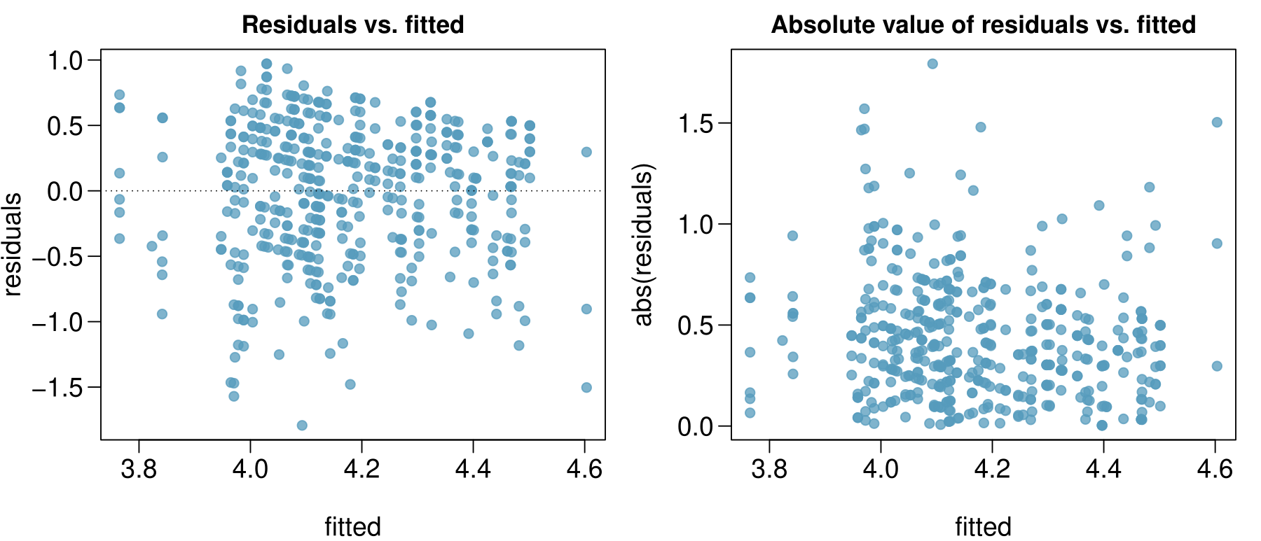
(2) constant variability in residuals
scatterplot of residuals and/or absolute value of residuals vs. fitted (predicted):
Does this condition appear to be satisfied?
Checking constant variance - recap
When we did simple linear regression (one explanatory variable) we checked the constant variance condition using a plot of residuals vs. x.
With multiple linear regression (2+ explanatory variables) we checked the constant variance condition using a plot of residuals vs. fitted.
\(\:\)
Why are we using different plots?
In multiple linear regression there are many explanatory variables, so a plot of residuals vs. one of them wouldn’t give us the complete picture.
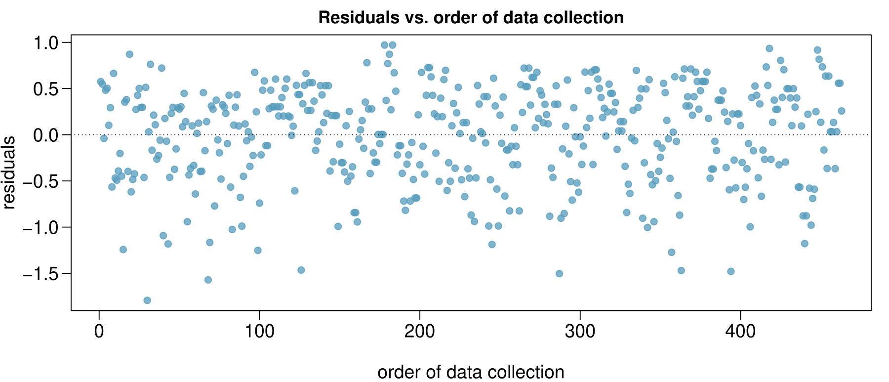
(3) independent residuals
scatterplot of residuals vs. order of data collection:
Does this condition appear to be satisfied?
More on the condition of independent residuals
Checking for independent residuals allows us to indirectly check for independent observations.
If observations and residuals are independent, we would not expect to see an increasing or decreasing trend in the scatterplot of residuals vs. order of data collection.
This condition is often violated when we have time series data. Such data require more advanced time series regression techniques for proper analysis.
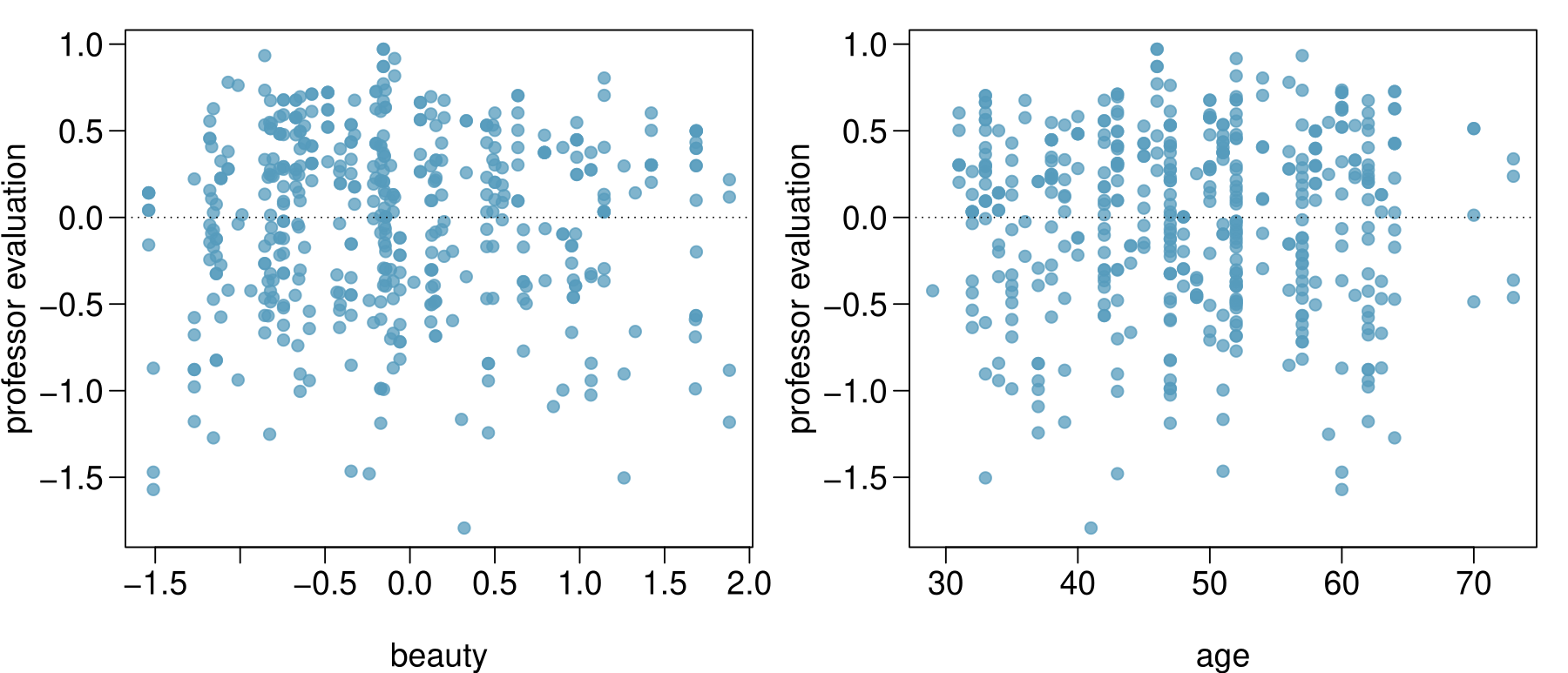
(4) linear relationships
scatterplot of residuals vs. each (numerical) explanatory variable:
Does this condition appear to be satisfied?
We use residuals instead of the predictors on the y-axis so that we can still check for linearity without worrying about other possible violations like collinearity between the predictors.
Several options for improving a model
Transforming variables
Seeking out additional variables to fill model gaps
Using more advanced methods that would account for challenges around inconsistent variability or nonlinear relationships between predictors and the outcome
Models can be wrong, but useful
All models are wrong, but some are useful. - George Box
No model is perfect, but even imperfect models can be useful, as long as we are clear and report the model’s shortcomings.
If conditions are grossly violated, we should not report the model results, but instead consider a new model, even if it means learning more statistical methods or asking someone for help.