Statistics for Analytics

Session 9: Model Checking & a Complete Analysis

Dr Zexun Chen

Zexun.Chen@ed.ac.uk

Today’s route

Interpret an adjusted model, check its behaviour and communicate a defensible analytical decision.

Teaching time: 110 minutes, plus a 10-minute break. The timed blocks include calculation, discussion and Wooclap debriefs.

• 000–005 min: Retrieve the simple and multiple regression questions
• 005–030 min: Reading and comparing adjusted models, including coefficient activity
• 030–055 min: Residual diagnostics, dependence and influence
• 055–065 min: Break
• 065–085 min: Model selection, transformations and validation
• 085–115 min: Integrated analysis: define, compare, check and recommend
• 115–120 min: Course synthesis and questions

Reference slides are available after the session takeaway and are not part of the core two-hour route.

Reading & Comparing Models

What the first model leaves to explain

The simple model from Session 8 estimates September bill using credit limit:

\[\widehat{\text{bill}}=24.09+1.620(\text{limit}),\qquad R^2=.0815.\]

Bill is in thousand NTD; limit is in units of 10,000 NTD.

Today’s question: can extra predictors improve the explanation, and what evidence would justify using the model for prediction?

Five-minute retrieval. Ask students to interpret the slope and distinguish low R-squared from absence of association. Recall the expanded model with age and repayment-group indicators introduced at the end of Session 8. The session develops conditional interpretation, diagnostics and validation before a 30-minute integrated analysis.

Credit-data example

Variable	Role	Unit
September bill	Response	Thousand NTD
Credit limit	Predictor	10,000 NTD
Age	Predictor	Years
Repayment-status group	Predictor	Two indicators; no recorded delay is the reference

The fitted sample contains all 30,000 published records.

Source: Yeh, UCI Default of Credit Card Clients. This model describes recorded September bills.

ANOVA and regression

ANOVA is a linear model with categorical predictors.

\[Y_i=\beta_0+\beta_1I(\text{University})+ \beta_2I(\text{High school})+\varepsilon_i\]

The coefficients compare each group with Graduate school, the reference category.

Interpret an adjusted comparison

The coefficient for two or more months late is +21.315, with bill in thousand NTD. What does it describe?

1. A 21.315% increase in default risk
2. An estimated 21,315 NTD higher mean bill than the reference group, holding limit and age fixed
3. A guaranteed 21,315 NTD increase for each client
4. The causal effect of delaying repayment

Allow 5 minutes within the multiple-regression block. Correct: option 2. Explain the reference group, holding included variables fixed, the response units and the observational scope. Ask why a repayment-status code needs category indicators rather than an assumed equally spaced scale.

Overall F-test

\[H_0:\beta_1=\cdots=\beta_p=0\]

\[F=\frac{SSR/p}{SSE/(n-p-1)}.\]

The test asks whether the predictors collectively improve on an intercept-only model.

Adjusted \(R^2\)

\[R^2_{adj}=1-(1-R^2)\frac{n-1}{n-p-1}.\]

Unlike \(R^2\), adjusted \(R^2\) penalises adding predictors that contribute little.

It is not a substitute for out-of-sample validation.

Model Diagnostics

Diagnose residual patterns

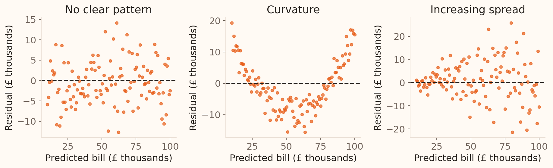
Pattern	What to investigate
Curve	Mean relationship, transformation, or missing terms
Funnel	Changing variance and the standard-error method

Illustrative bill-model simulations, seed 202609.

Also inspect clusters and extreme residuals. They can suggest omitted groups, dependence, data errors, or influential observations. For changing variance, consider a suitable transformation, robust standard errors, or a model for the variance, according to the analytical purpose.

Normal residuals

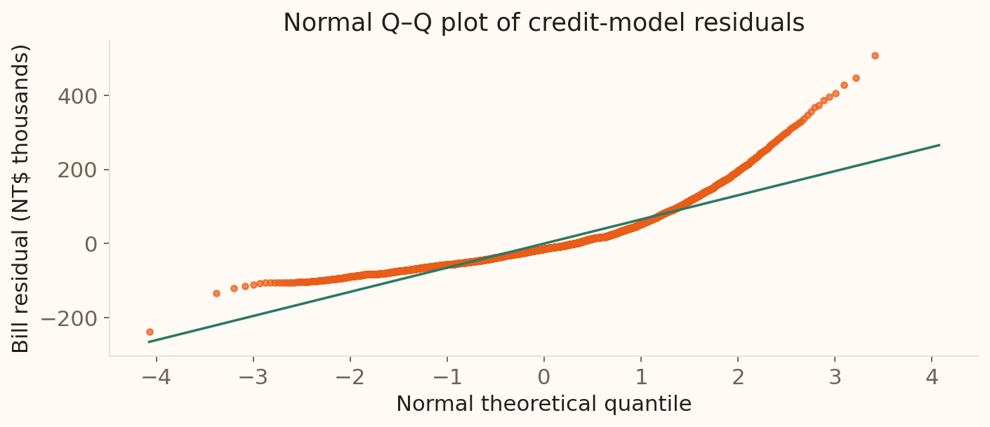
The heavy tails deserve investigation. Normality matters most for exact small-sample inference.

UCI Default of Credit Card Clients. Residuals from the model fitted to all 30,000 records; plotted quantiles are thinned for legibility.

Independence

Plot residuals in time or collection order.

Patterns may indicate:

• seasonality;
• serial correlation;
• repeated observations;
• omitted process changes.

Dependence requires a model that reflects the data structure.

Outlier, leverage, influence

Concept	Unusual in…	Main concern
Outlier	Response direction	Large residual
High leverage	Predictor space	Can pull the line
Influential point	Fitted result	Changes estimates materially

Influence combines position and residual size.

Which point changes the fitted line?

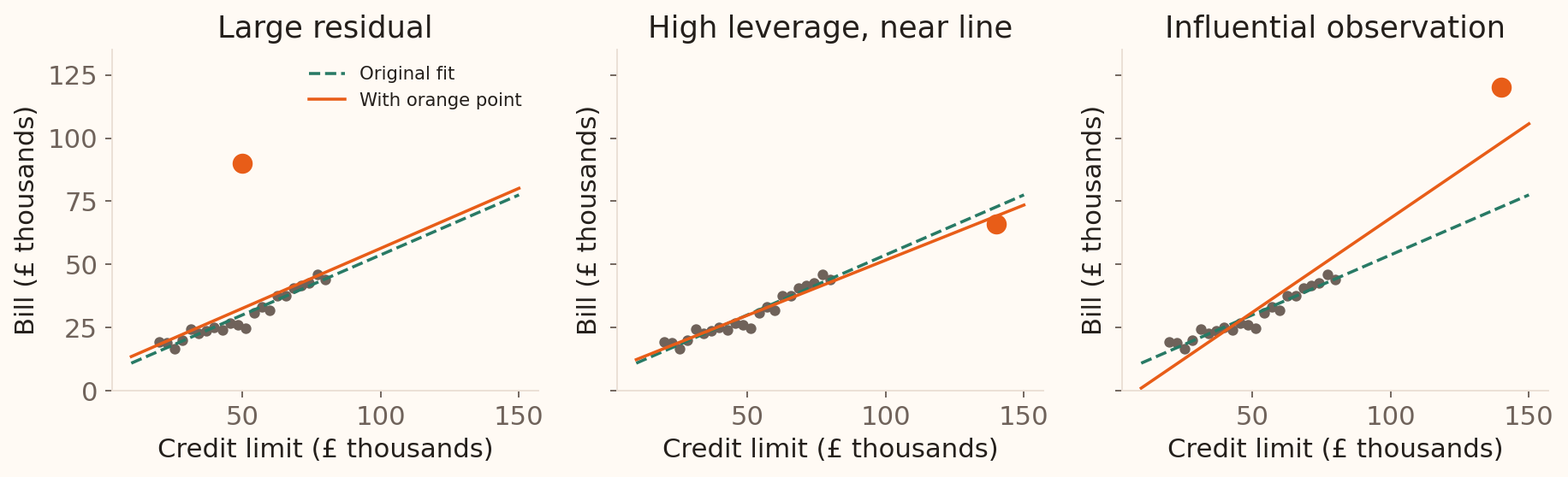
Verify the record, understand its context, compare fits with and without it, and report sensitivity.

Illustrative data, seed 202609. Green dashed line: original fit. Orange line: fit including the highlighted point.

Collinearity

Highly related predictors make individual coefficients unstable.

Signs include:

• large standard errors;
• coefficients changing with small model changes;
• high variance inflation factors;
• strong predictor correlations.

Prediction may remain adequate even when interpretation is unstable.

Building & Validating

Selecting predictors

Strategy	Start	Next step
Forward selection	A baseline model	Add a justified predictor and reassess
Backward elimination	A candidate full model	Remove a predictor and reassess

Compare adjusted \(R^2\), validation error, and interpretability. Preserve variables required by the scientific question.

The original lecture presents selection by adjusted R-squared and by p-values. With adjusted R-squared, compare candidate additions or deletions and stop when none improves the criterion. A p-value approach adds significant candidates or removes the least significant term and refits. Repeated search changes the interpretation of ordinary post-selection p-values, so it should not be treated as a guarantee of a correct model. Perform selection within the training/validation process, keeping the final test data untouched.

Prediction needs validation

Train

Estimate model

Validate

Tune choices

Test

Final performance

Monitor

Drift after launch

Never evaluate predictive performance only on the fitting data.

Choose metrics for the decision

Goal	Possible metric
Penalise large errors	RMSE
Robust typical error	MAE
Explain in-sample variation	\(R^2\)
Compare likelihood models	AIC/BIC

No single metric answers every modelling question.

Transformations

Transform when theory and diagnostics support it.

Pattern	Possible response
Strictly positive, right-skewed outcome	\(\log Y\)
Multiplicative effect	\(\log Y\) or \(\log X\)
Curvature	Polynomial, spline, transform
Changing variance	Transform or robust SE

Interpret transformed coefficients on the transformed scale.

Some recorded bills are zero or negative, so a direct log transformation is undefined for them.

A Complete Analysis

Analysis workshop: define the decision

A bank team wants to understand September bills and assess whether the analysis could support later predictions.

Available evidence	Scope
30,000 credit-card records	One published historical dataset
Limit, age and September repayment status	Candidate predictors
September bill	Numerical outcome

Define the observational unit, response and units. Which predictors would be available at the intended prediction time?

Workshop stage 1, 8 minutes: 4 minutes in pairs, 4 minutes discussion. Unit: one account/client record. Response: September bill in thousand NTD. Limit is measured in units of 10,000 NTD in these regressions, age in years and status through two indicators. A retrospective explanation can use recorded September status. For a forecast made before September, verify what is available; information from within or after the outcome period can cause leakage. The dataset supports this historical analysis; claims about future cohorts require suitable later data. The lecture exercise uses the supplied evidence rather than live model fitting.

Analysis workshop: compare the evidence

Result	Credit limit alone	Limit, age and status group
Limit slope (NTD per 10,000 NTD)	1,620	1,659
\(R^2\)	.0815	.1007
Adjusted \(R^2\)	.0814	.1006

1. Interpret the adjusted limit slope.
2. Describe how much the observed fit improves.
3. Identify what these results leave unanswered about prediction.

Workshop stage 2, 10 minutes: 5 minutes discussion, 3 minutes drafting a comparison, 2 minutes reporting. The adjusted association is 1,659 NTD higher mean bill per 10,000 NTD of limit at the same age and status. R-squared rises about 1.92 percentage points, with most bill variation still unexplained. In-sample improvement does not establish held-out prediction, valid conventional SEs or causality. Adjusted R-squared values use n = 30,000 and 1 or 4 slopes: .0814396 and .1005626. Source: the verified UCI regressions from the earlier slides.

Analysis workshop: choose the next checks

The simple model has changing residual spread and heavy tails. Some recorded bills are zero or negative.

Propose a short analysis plan covering:

1. Diagnostics for the expanded model and treatment of unusual records.
2. A justified transformation or uncertainty method.
3. Validation data, an error metric and one limit on the claim.

Workshop stage 3, 7 minutes: 4 minutes planning, 3 minutes sharing. Recompute residual-versus-fitted and Q–Q plots for the expanded model, inspect influential records and investigate data meaning before deletion. Direct log(Y) is undefined for nonpositive bills; use a justified compatible transformation, model or robust uncertainty method. Separate fitting and selection from final evaluation. Choose MAE or RMSE from the decision and compare a simple benchmark. A held-out subset of this cohort tests generalisation to similar accounts; a future-cohort forecast needs later data and predictor availability checks. Use the final Wooclap for a 5-minute recommendation and debrief to complete the 30 minutes.

Is this model ready for prediction?

Submit a three-sentence recommendation: what the banking models show, which checks or validation are needed, and what decision the evidence currently supports.

Format: open response; final five-minute workshop debrief. Expected: inspect mean form and variance, assess important predictors and influential records, consider transformations compatible with zero/negative bills, and evaluate predictions on held-out data reflecting the intended use. Ask students to distinguish better fit from reliable prediction.

Session 9 takeaway

• Interpret coefficients conditional on the included predictors.
• Use residuals, data context and sensitivity checks to diagnose a model.
• Keep model selection separate from final performance evaluation.
• Communicate the question, evidence, uncertainty and next action.

Bring unresolved method and reporting questions to the course Q&A.

Reference

Models are useful simplifications

Judge a model by its purpose, assumptions, validation, interpretability, and consequences.